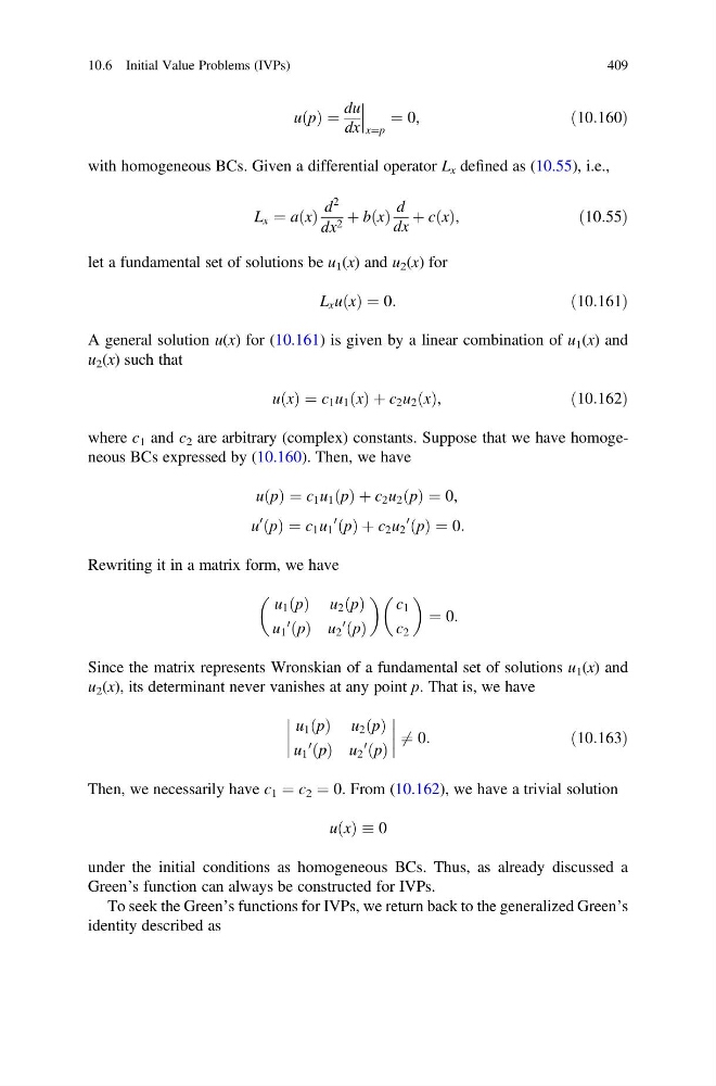
u p
ð Þ ¼
du
dx
x¼p
¼ 0,
ð10:160Þ
with homogeneous BCs. Given a differential operator L x defined as (10.55), i.e.,
L x ¼ a x
ð Þ
d
2
dx 2 þ b x
ð Þ
d
dx
þ c x
ð Þ,
ð10:55Þ
let a fundamental set of solutions be u 1 (x) and u 2 (x) for
L x u x
ð Þ ¼ 0:
ð10:161Þ
A general solution u(x) for (10.161) is given by a linear combination of u 1 (x) and
u 2 (x) such that
u x
ð Þ ¼ c 1 u 1 x
ð Þ þ c 2 u 2 x
ð Þ,
ð10:162Þ
where c 1 and c 2 are arbitrary (complex) constants. Suppose that we have homogeneous BCs expressed by (10.160). Then, we have
u p
ð Þ ¼ c 1 u 1 p
ð Þ þ c 2 u 2 p
ð Þ ¼ 0,
u
0 p
ð Þ ¼ c 1 u 1
0 p
ð Þ þ c 2 u 2
0 p
ð Þ ¼ 0:
Rewriting it in a matrix form, we have
u 1 p
ð Þ u 2 p
ð Þ
u 1
0 p
ð Þ u 2
0 p
ð Þ
c 1
c 2
¼ 0:
Since the matrix represents Wronskian of a fundamental set of solutions u 1 (x) and
u 2 (x), its determinant never vanishes at any point p. That is, we have
u 1 p
ð Þ u 2 p
ð Þ
u 1
0 p
ð Þ u 2
0 p
ð Þ
6 ¼ 0:
ð10:163Þ
Then, we necessarily have c 1 ¼ c 2 ¼ 0. From (10.162), we have a trivial solution
u x
ð Þ 0
under the initial conditions as homogeneous BCs. Thus, as already discussed a
Green’s function can always be constructed for IVPs.
To seek the Green’s functions for IVPs, we return back to the generalized Green’s
identity described as
10.6 Initial Value Problems (IVPs)
409