

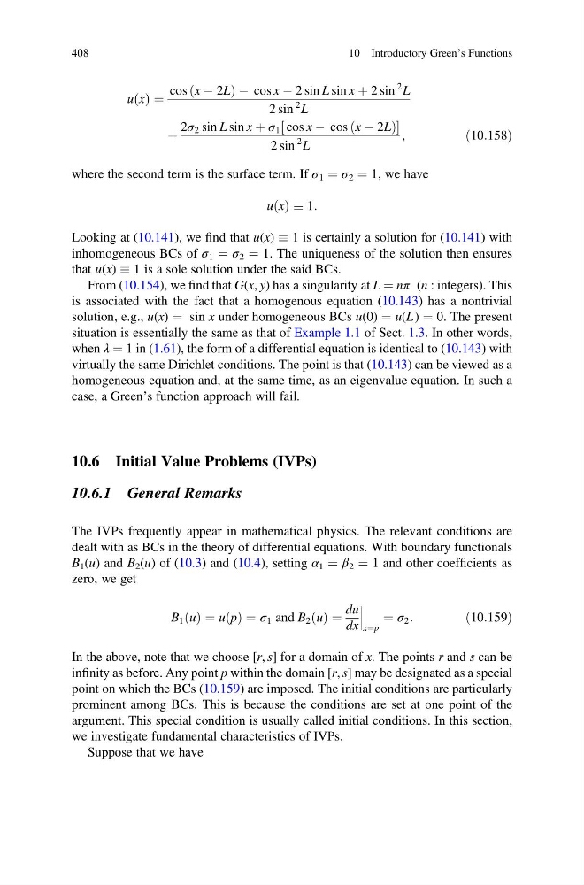
u x
ð Þ ¼
cos x À 2L
ð
ÞÀ cos x À 2 sin L sin x þ 2 sin
2 L
2 sin
2 L
þ
2σ 2 sin L sin x þ σ 1 cos x À cos x À 2L
ð
Þ
½
2 sin
2 L
,
ð10:158Þ
where the second term is the surface term. If σ 1 ¼ σ 2 ¼ 1, we have
u x
ð Þ 1:
Looking at (10.141), we find that u(x) 1 is certainly a solution for (10.141) with
inhomogeneous BCs of σ 1 ¼ σ 2 ¼ 1. The uniqueness of the solution then ensures
that u(x) 1 is a sole solution under the said BCs.
From (10.154), we find that G(x, y) has a singularity at L ¼ nπ (n : integers). This
is associated with the fact that a homogenous equation (10.143) has a nontrivial
solution, e.g., u(x) ¼ sin x under homogeneous BCs u(0) ¼ u(L ) ¼ 0. The present
situation is essentially the same as that of Example 1.1 of Sect. 1.3. In other words,
when λ ¼ 1 in (1.61), the form of a differential equation is identical to (10.143) with
virtually the same Dirichlet conditions. The point is that (10.143) can be viewed as a
homogeneous equation and, at the same time, as an eigenvalue equation. In such a
case, a Green’s function approach will fail.
10.6 Initial Value Problems (IVPs)
10.6.1 General Remarks
The IVPs frequently appear in mathematical physics. The relevant conditions are
dealt with as BCs in the theory of differential equations. With boundary functionals
B 1 (u) and B 2 (u) of (10.3) and (10.4), setting α 1 ¼ β 2 ¼ 1 and other coefficients as
zero, we get
B 1 u
ð Þ ¼ u p
ð Þ ¼ σ 1 and B 2 u
ð Þ ¼
du
dx
x¼p
¼ σ 2 :
ð10:159Þ
In the above, note that we choose [r, s] for a domain of x. The points r and s can be
infinity as before. Any point p within the domain [r, s] may be designated as a special
point on which the BCs (10.159) are imposed. The initial conditions are particularly
prominent among BCs. This is because the conditions are set at one point of the
argument. This special condition is usually called initial conditions. In this section,
we investigate fundamental characteristics of IVPs.
Suppose that we have
408
10 Introductory Green’s Functions
ð Þ ¼
cos x À 2L
ð
ÞÀ cos x À 2 sin L sin x þ 2 sin
2 L
2 sin
2 L
þ
2σ 2 sin L sin x þ σ 1 cos x À cos x À 2L
ð
Þ
½
2 sin
2 L
,
ð10:158Þ
where the second term is the surface term. If σ 1 ¼ σ 2 ¼ 1, we have
u x
ð Þ 1:
Looking at (10.141), we find that u(x) 1 is certainly a solution for (10.141) with
inhomogeneous BCs of σ 1 ¼ σ 2 ¼ 1. The uniqueness of the solution then ensures
that u(x) 1 is a sole solution under the said BCs.
From (10.154), we find that G(x, y) has a singularity at L ¼ nπ (n : integers). This
is associated with the fact that a homogenous equation (10.143) has a nontrivial
solution, e.g., u(x) ¼ sin x under homogeneous BCs u(0) ¼ u(L ) ¼ 0. The present
situation is essentially the same as that of Example 1.1 of Sect. 1.3. In other words,
when λ ¼ 1 in (1.61), the form of a differential equation is identical to (10.143) with
virtually the same Dirichlet conditions. The point is that (10.143) can be viewed as a
homogeneous equation and, at the same time, as an eigenvalue equation. In such a
case, a Green’s function approach will fail.
10.6 Initial Value Problems (IVPs)
10.6.1 General Remarks
The IVPs frequently appear in mathematical physics. The relevant conditions are
dealt with as BCs in the theory of differential equations. With boundary functionals
B 1 (u) and B 2 (u) of (10.3) and (10.4), setting α 1 ¼ β 2 ¼ 1 and other coefficients as
zero, we get
B 1 u
ð Þ ¼ u p
ð Þ ¼ σ 1 and B 2 u
ð Þ ¼
du
dx
x¼p
¼ σ 2 :
ð10:159Þ
In the above, note that we choose [r, s] for a domain of x. The points r and s can be
infinity as before. Any point p within the domain [r, s] may be designated as a special
point on which the BCs (10.159) are imposed. The initial conditions are particularly
prominent among BCs. This is because the conditions are set at one point of the
argument. This special condition is usually called initial conditions. In this section,
we investigate fundamental characteristics of IVPs.
Suppose that we have
408
10 Introductory Green’s Functions