f x
ð Þ δ x
ð Þ ¼ f 0
ð Þ δ x
ð Þ or f x
ð Þ δ x À y
ð
Þ¼f y
ð Þ δ x À y
ð
Þ,
ð10:116Þ
we have
∂
∂x
p
∂G
∂x
¼
p y
ð Þ
a y
ð Þ
δ x À y
ð
Þ
w y
ð Þ
À
p x
ð Þc x
ð Þ
a x
ð Þ
G x, y
ð Þ:
ð10:117Þ
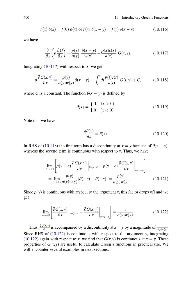
Integrating (10.117) with respect to x, we get
p
∂G x, y
ð Þ
∂x
¼
p y
ð Þ
a y
ð Þw y
ð Þ
θ x À y
ð
ÞÀ
Z x
r
dt
p t
ð Þc t
ð Þ
a t
ð Þ
G t, y
ð Þ þ C,
ð10:118Þ
where C is a constant. The function θ(x À y) is defined by
θ x
ð Þ ¼
1 x > 0
ð
Þ
0 x < 0
ð
Þ:
&
ð10:119Þ
Note that we have
dθ x
ð Þ
dx
¼ δ x
ð Þ:
ð10:120Þ
In RHS of (10.118) the first term has a discontinuity at x ¼ y because of θ(x À y),
whereas the second term is continuous with respect to y. Thus, we have
lim
ε!þ0
p y þ ε
ð
Þ
∂G x, y
ð Þ
∂x
x¼yþε À p y À ε
ð
Þ
∂G x, y
ð Þ
∂x
x¼yÀε
"
#
¼ lim
ε!þ0
p y
ð Þ
a y
ð Þw y
ð Þ
θ þε
ð Þ À θ Àε
ð Þ
½
Š ¼
p y
ð Þ
a y
ð Þw y
ð Þ
:
ð10:121Þ
Since p( y) is continuous with respect to the argument y, this factor drops off and we
get
lim
ε!þ0
∂G x, y
ð Þ
∂x
x¼yþε À
∂G x, y
ð Þ
∂x
x¼yÀε
"
#
¼
1
a y
ð Þw y
ð Þ
:
ð10:122Þ
Thus,
∂G x, y
ð Þ
∂x
is accompanied by a discontinuity at x ¼ y by a magnitude of
1
a y
ð Þw y
ð Þ .
Since RHS of (10.122) is continuous with respect to the argument y, integrating
(10.122) again with respect to x, we find that G(x, y) is continuous at x ¼ y. These
properties of G(x, y) are useful to calculate Green’s functions in practical use. We
will encounter several examples in next sections.
400
10 Introductory Green’s Functions