

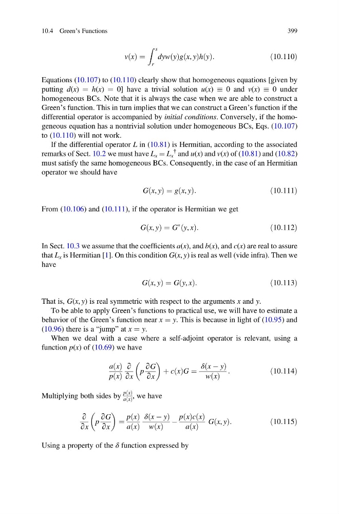
v x
ð Þ ¼
Z s
r
dyw y
ð Þg x, y
ð Þh y
ð Þ:
ð10:110Þ
Equations (10.107) to (10.110) clearly show that homogeneous equations [given by
putting d(x) ¼ h(x) ¼ 0] have a trivial solution u(x) 0 and v(x) 0 under
homogeneous BCs. Note that it is always the case when we are able to construct a
Green’s function. This in turn implies that we can construct a Green’s function if the
differential operator is accompanied by initial conditions. Conversely, if the homogeneous equation has a nontrivial solution under homogeneous BCs, Eqs. (10.107)
to (10.110) will not work.
If the differential operator L in (10.81) is Hermitian, according to the associated
remarks of Sect. 10.2 we must have L x ¼ L x
{ and u(x) and v(x) of (10.81) and (10.82)
must satisfy the same homogeneous BCs. Consequently, in the case of an Hermitian
operator we should have
G x, y
ð Þ ¼ g x, y
ð Þ:
ð10:111Þ
From (10.106) and (10.111), if the operator is Hermitian we get
G x, y
ð Þ ¼ G
à y, x
ð Þ:
ð10:112Þ
In Sect. 10.3 we assume that the coefficients a(x), and b(x), and c(x) are real to assure
that L x is Hermitian [1]. On this condition G(x, y) is real as well (vide infra). Then we
have
G x, y
ð Þ ¼ G y, x
ð Þ:
ð10:113Þ
That is, G(x, y) is real symmetric with respect to the arguments x and y.
To be able to apply Green’s functions to practical use, we will have to estimate a
behavior of the Green’s function near x ¼ y. This is because in light of (10.95) and
(10.96) there is a “jump” at x ¼ y.
When we deal with a case where a self-adjoint operator is relevant, using a
function p(x) of (10.69) we have
a x
ð Þ
p x
ð Þ
∂
∂x
p
∂G
∂x
þ c x
ð ÞG ¼
δ x À y
ð
Þ
w x
ð Þ
:
ð10:114Þ
Multiplying both sides by
p x
ð Þ
a x
ð Þ , we have
∂
∂x
p
∂G
∂x
¼
p x
ð Þ
a x
ð Þ
δ x À y
ð
Þ
w x
ð Þ
À
p x
ð Þc x
ð Þ
a x
ð Þ
G x, y
ð Þ:
ð10:115Þ
Using a property of the δ function expressed by
10.4 Green’s Functions
399
ð Þ ¼
Z s
r
dyw y
ð Þg x, y
ð Þh y
ð Þ:
ð10:110Þ
Equations (10.107) to (10.110) clearly show that homogeneous equations [given by
putting d(x) ¼ h(x) ¼ 0] have a trivial solution u(x) 0 and v(x) 0 under
homogeneous BCs. Note that it is always the case when we are able to construct a
Green’s function. This in turn implies that we can construct a Green’s function if the
differential operator is accompanied by initial conditions. Conversely, if the homogeneous equation has a nontrivial solution under homogeneous BCs, Eqs. (10.107)
to (10.110) will not work.
If the differential operator L in (10.81) is Hermitian, according to the associated
remarks of Sect. 10.2 we must have L x ¼ L x
{ and u(x) and v(x) of (10.81) and (10.82)
must satisfy the same homogeneous BCs. Consequently, in the case of an Hermitian
operator we should have
G x, y
ð Þ ¼ g x, y
ð Þ:
ð10:111Þ
From (10.106) and (10.111), if the operator is Hermitian we get
G x, y
ð Þ ¼ G
à y, x
ð Þ:
ð10:112Þ
In Sect. 10.3 we assume that the coefficients a(x), and b(x), and c(x) are real to assure
that L x is Hermitian [1]. On this condition G(x, y) is real as well (vide infra). Then we
have
G x, y
ð Þ ¼ G y, x
ð Þ:
ð10:113Þ
That is, G(x, y) is real symmetric with respect to the arguments x and y.
To be able to apply Green’s functions to practical use, we will have to estimate a
behavior of the Green’s function near x ¼ y. This is because in light of (10.95) and
(10.96) there is a “jump” at x ¼ y.
When we deal with a case where a self-adjoint operator is relevant, using a
function p(x) of (10.69) we have
a x
ð Þ
p x
ð Þ
∂
∂x
p
∂G
∂x
þ c x
ð ÞG ¼
δ x À y
ð
Þ
w x
ð Þ
:
ð10:114Þ
Multiplying both sides by
p x
ð Þ
a x
ð Þ , we have
∂
∂x
p
∂G
∂x
¼
p x
ð Þ
a x
ð Þ
δ x À y
ð
Þ
w x
ð Þ
À
p x
ð Þc x
ð Þ
a x
ð Þ
G x, y
ð Þ:
ð10:115Þ
Using a property of the δ function expressed by
10.4 Green’s Functions
399