

cos kL ¼ 0:
ð1:80Þ
Hence,
kL ¼
π
2
þ mπ m ¼ 0, Æ1, Æ2, Á Á Á
ð
Þ :
ð1:81Þ
In (1.81), for instance, we have k ¼
π
2L for m ¼ 0 and k ¼ À
π
2L for m ¼ À 1. Also, we
have k ¼
3π
2L for m ¼ 1 and k ¼ À
3π
2L for m ¼ À 2. These cases, however, individually
give linearly dependent solutions for (1.78). Therefore, to get a set of linearly
independent eigenfunctions we may define k as positive. Correspondingly, from
(1.68) we get eigenvalues of
λ ¼ 2m þ 1
ð
Þ
2 π
2
=4L
2 m ¼ 0, 1, 2, Á Á Á
ð
Þ :
ð1:82Þ
Also, inserting BCs (1.62) into (1.79), we have
sin kL ¼ 0:
ð1:83Þ
Hence,
kL ¼ nπ n ¼ 1, 2, 3, Á Á Á
ð
Þ :
ð1:84Þ
From (1.68) we get
λ ¼ n
2
π
2
=L
2
¼ 2n
ð Þ
2 π
2
=4L
2 n ¼ 1, 2, 3, Á Á Á
ð
Þ ,
ð1:85Þ
where we chose positive numbers n for the same reason as the above. With the
second equality of (1.85), we made eigenvalues easily comparable to those of (1.82).
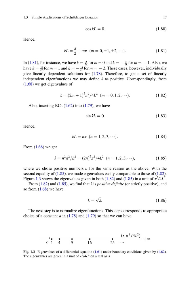
Figure 1.3 shows the eigenvalues given in both (1.82) and (1.85) in a unit of π
2 /4L
2 .
From (1.82) and (1.85), we find that λ is positive definite (or strictly positive), and
so from (1.68) we have
k ¼
ffiffi ffi
λ
p :
ð1:86Þ
The next step is to normalize eigenfunctions. This step corresponds to appropriate
choice of a constant a in (1.78) and (1.79) so that we can have
[ /4 +∞
⋯
0 1
9
25
16
4
Fig. 1.3 Eigenvalues of a differential equation (1.61) under boundary conditions given by (1.62).
The eigenvalues are given in a unit of π
2
/4L
2 on a real axis
1.3 Simple Applications of Schrödinger Equation
17
ð1:80Þ
Hence,
kL ¼
π
2
þ mπ m ¼ 0, Æ1, Æ2, Á Á Á
ð
Þ :
ð1:81Þ
In (1.81), for instance, we have k ¼
π
2L for m ¼ 0 and k ¼ À
π
2L for m ¼ À 1. Also, we
have k ¼
3π
2L for m ¼ 1 and k ¼ À
3π
2L for m ¼ À 2. These cases, however, individually
give linearly dependent solutions for (1.78). Therefore, to get a set of linearly
independent eigenfunctions we may define k as positive. Correspondingly, from
(1.68) we get eigenvalues of
λ ¼ 2m þ 1
ð
Þ
2 π
2
=4L
2 m ¼ 0, 1, 2, Á Á Á
ð
Þ :
ð1:82Þ
Also, inserting BCs (1.62) into (1.79), we have
sin kL ¼ 0:
ð1:83Þ
Hence,
kL ¼ nπ n ¼ 1, 2, 3, Á Á Á
ð
Þ :
ð1:84Þ
From (1.68) we get
λ ¼ n
2
π
2
=L
2
¼ 2n
ð Þ
2 π
2
=4L
2 n ¼ 1, 2, 3, Á Á Á
ð
Þ ,
ð1:85Þ
where we chose positive numbers n for the same reason as the above. With the
second equality of (1.85), we made eigenvalues easily comparable to those of (1.82).
Figure 1.3 shows the eigenvalues given in both (1.82) and (1.85) in a unit of π
2 /4L
2 .
From (1.82) and (1.85), we find that λ is positive definite (or strictly positive), and
so from (1.68) we have
k ¼
ffiffi ffi
λ
p :
ð1:86Þ
The next step is to normalize eigenfunctions. This step corresponds to appropriate
choice of a constant a in (1.78) and (1.79) so that we can have
[ /4 +∞
⋯
0 1
9
25
16
4
Fig. 1.3 Eigenvalues of a differential equation (1.61) under boundary conditions given by (1.62).
The eigenvalues are given in a unit of π
2
/4L
2 on a real axis
1.3 Simple Applications of Schrödinger Equation
17