

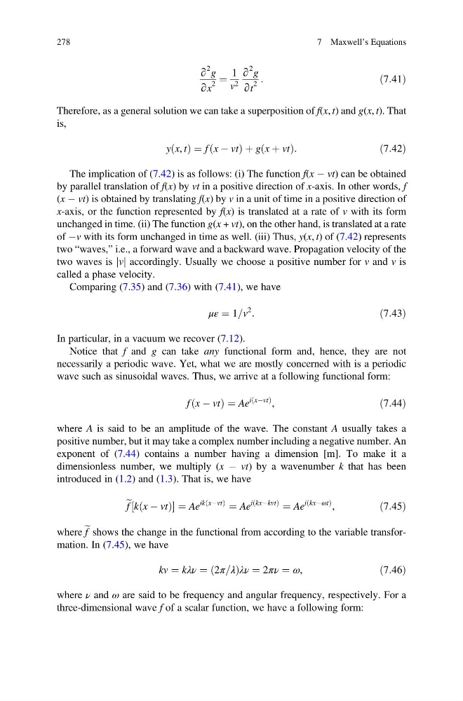
∂
2 g
∂x
2
¼
1
v 2
∂
2 g
∂t
2
:
ð7:41Þ
Therefore, as a general solution we can take a superposition of f(x, t) and g(x, t). That
is,
y x, t
ð Þ ¼ f x À vt
ð
Þþg x þ vt
ð
Þ:
ð7:42Þ
The implication of (7.42) is as follows: (i) The function f(x À vt) can be obtained
by parallel translation of f(x) by vt in a positive direction of x-axis. In other words, f
(x À vt) is obtained by translating f(x) by v in a unit of time in a positive direction of
x-axis, or the function represented by f(x) is translated at a rate of v with its form
unchanged in time. (ii) The function g(x + vt), on the other hand, is translated at a rate
of Àv with its form unchanged in time as well. (iii) Thus, y(x, t) of (7.42) represents
two “waves,” i.e., a forward wave and a backward wave. Propagation velocity of the
two waves is jvj accordingly. Usually we choose a positive number for v and v is
called a phase velocity.
Comparing (7.35) and (7.36) with (7.41), we have
με ¼ 1=v
2
:
ð7:43Þ
In particular, in a vacuum we recover (7.12).
Notice that f and g can take any functional form and, hence, they are not
necessarily a periodic wave. Yet, what we are mostly concerned with is a periodic
wave such as sinusoidal waves. Thus, we arrive at a following functional form:
f x À vt
ð
Þ¼Ae
i xÀvt
ð
Þ ,
ð7:44Þ
where A is said to be an amplitude of the wave. The constant A usually takes a
positive number, but it may take a complex number including a negative number. An
exponent of (7.44) contains a number having a dimension [m]. To make it a
dimensionless number, we multiply (x À vt) by a wavenumber k that has been
introduced in (1.2) and (1.3). That is, we have
e f k x À vt
ð
Þ
½
¼Ae
ik xÀvt
ð
Þ
¼ Ae
i kxÀkvt
ð
Þ
¼ Ae
i kxÀωt
ð
Þ ,
ð7:45Þ
where e f shows the change in the functional from according to the variable transformation. In (7.45), we have
kv ¼ kλν ¼ 2π=λ
ð
Þλν ¼ 2πν ¼ ω,
ð7:46Þ
where ν and ω are said to be frequency and angular frequency, respectively. For a
three-dimensional wave f of a scalar function, we have a following form:
278
7 Maxwell’s Equations
2 g
∂x
2
¼
1
v 2
∂
2 g
∂t
2
:
ð7:41Þ
Therefore, as a general solution we can take a superposition of f(x, t) and g(x, t). That
is,
y x, t
ð Þ ¼ f x À vt
ð
Þþg x þ vt
ð
Þ:
ð7:42Þ
The implication of (7.42) is as follows: (i) The function f(x À vt) can be obtained
by parallel translation of f(x) by vt in a positive direction of x-axis. In other words, f
(x À vt) is obtained by translating f(x) by v in a unit of time in a positive direction of
x-axis, or the function represented by f(x) is translated at a rate of v with its form
unchanged in time. (ii) The function g(x + vt), on the other hand, is translated at a rate
of Àv with its form unchanged in time as well. (iii) Thus, y(x, t) of (7.42) represents
two “waves,” i.e., a forward wave and a backward wave. Propagation velocity of the
two waves is jvj accordingly. Usually we choose a positive number for v and v is
called a phase velocity.
Comparing (7.35) and (7.36) with (7.41), we have
με ¼ 1=v
2
:
ð7:43Þ
In particular, in a vacuum we recover (7.12).
Notice that f and g can take any functional form and, hence, they are not
necessarily a periodic wave. Yet, what we are mostly concerned with is a periodic
wave such as sinusoidal waves. Thus, we arrive at a following functional form:
f x À vt
ð
Þ¼Ae
i xÀvt
ð
Þ ,
ð7:44Þ
where A is said to be an amplitude of the wave. The constant A usually takes a
positive number, but it may take a complex number including a negative number. An
exponent of (7.44) contains a number having a dimension [m]. To make it a
dimensionless number, we multiply (x À vt) by a wavenumber k that has been
introduced in (1.2) and (1.3). That is, we have
e f k x À vt
ð
Þ
½
¼Ae
ik xÀvt
ð
Þ
¼ Ae
i kxÀkvt
ð
Þ
¼ Ae
i kxÀωt
ð
Þ ,
ð7:45Þ
where e f shows the change in the functional from according to the variable transformation. In (7.45), we have
kv ¼ kλν ¼ 2π=λ
ð
Þλν ¼ 2πν ¼ ω,
ð7:46Þ
where ν and ω are said to be frequency and angular frequency, respectively. For a
three-dimensional wave f of a scalar function, we have a following form:
278
7 Maxwell’s Equations