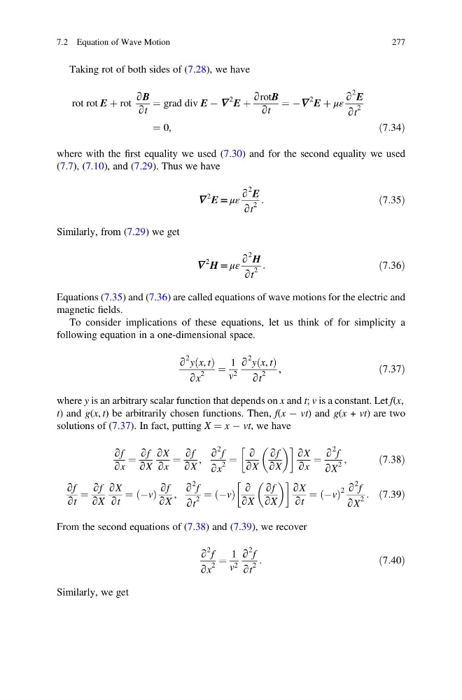
Taking rot of both sides of (7.28), we have
rot rot E þ rot
∂B
∂t
¼ grad div E À —
2 E þ
∂rotB
∂t
¼ À—
2 E þ με
∂
2 E
∂t
2
¼ 0,
ð7:34Þ
where with the first equality we used (7.30) and for the second equality we used
(7.7), (7.10), and (7.29). Thus we have
—
2 E = με
∂
2 E
∂t
2
:
ð7:35Þ
Similarly, from (7.29) we get
—
2 H = με
∂
2 H
∂t
2
:
ð7:36Þ
Equations (7.35) and (7.36) are called equations of wave motions for the electric and
magnetic fields.
To consider implications of these equations, let us think of for simplicity a
following equation in a one-dimensional space.
∂
2 y x, t
ð Þ
∂x
2
¼
1
v 2
∂
2 y x, t
ð Þ
∂t
2
,
ð7:37Þ
where y is an arbitrary scalar function that depends on x and t; v is a constant. Let f(x,
t) and g(x, t) be arbitrarily chosen functions. Then, f(x À vt) and g(x + vt) are two
solutions of (7.37). In fact, putting X ¼ x À vt, we have
∂f
∂x
¼
∂f
∂X
∂X
∂x
¼
∂f
∂X
,
∂
2 f
∂x
2
¼
∂
∂X
∂f
∂X
! ∂X
∂x
¼
∂
2 f
∂X
2
,
ð7:38Þ
∂f
∂t
¼
∂f
∂X
∂X
∂t
¼ Àv
ð Þ
∂f
∂X
,
∂
2 f
∂t
2
¼ Àv
ð Þ
∂
∂X
∂f
∂X
! ∂X
∂t
¼ Àv
ð Þ
2 ∂
2 f
∂X
2
: ð7:39Þ
From the second equations of (7.38) and (7.39), we recover
∂
2 f
∂x
2
¼
1
v 2
∂
2 f
∂t
2
:
ð7:40Þ
Similarly, we get
7.2 Equation of Wave Motion
277