

that is directed toward the upper side of the plane of paper (i.e., the positive direction
of the z-axis).
Equation (7.4) can be rewritten as
rot H ¼ i þ
∂D
∂t
:
ð7:16Þ
Notice that
∂D
∂t
has the same dimension as
A
m 2
Â
] and is called displacement current.
Without this term, we have
rot H ¼ i:
ð7:17Þ
This relation is well known as Ampère’s law or Ampère’s circuital law (André-Marie Ampère: 1827), which determines a magnetic field yielded by a stationary
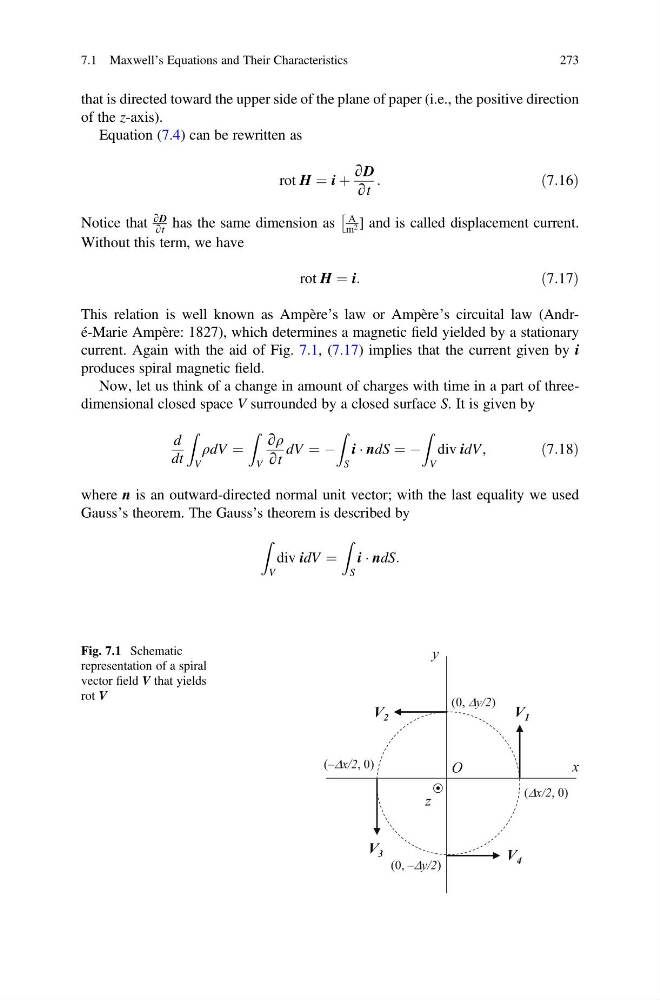
current. Again with the aid of Fig. 7.1, (7.17) implies that the current given by i
produces spiral magnetic field.
Now, let us think of a change in amount of charges with time in a part of threedimensional closed space V surrounded by a closed surface S. It is given by
d
dt
Z
V
ρdV ¼
Z
V
∂ρ
∂t
dV ¼ À
Z
S
i Á ndS ¼ À
Z
V
div idV,
ð7:18Þ
where n is an outward-directed normal unit vector; with the last equality we used
Gauss’s theorem. The Gauss’s theorem is described by
Z
V
div idV ¼
Z
S
i Á ndS:
x
y
V 1
V 2
V 3
V 4
O
(Δx/2, 0)
(‒Δx/2, 0)
(0, ‒Δy/2)
(0, Δy/2)
z
Fig. 7.1 Schematic
representation of a spiral
vector field V that yields
rot V
7.1 Maxwell’s Equations and Their Characteristics
273
of the z-axis).
Equation (7.4) can be rewritten as
rot H ¼ i þ
∂D
∂t
:
ð7:16Þ
Notice that
∂D
∂t
has the same dimension as
A
m 2
Â
] and is called displacement current.
Without this term, we have
rot H ¼ i:
ð7:17Þ
This relation is well known as Ampère’s law or Ampère’s circuital law (André-Marie Ampère: 1827), which determines a magnetic field yielded by a stationary
current. Again with the aid of Fig. 7.1, (7.17) implies that the current given by i
produces spiral magnetic field.
Now, let us think of a change in amount of charges with time in a part of threedimensional closed space V surrounded by a closed surface S. It is given by
d
dt
Z
V
ρdV ¼
Z
V
∂ρ
∂t
dV ¼ À
Z
S
i Á ndS ¼ À
Z
V
div idV,
ð7:18Þ
where n is an outward-directed normal unit vector; with the last equality we used
Gauss’s theorem. The Gauss’s theorem is described by
Z
V
div idV ¼
Z
S
i Á ndS:
x
y
V 1
V 2
V 3
V 4
O
(Δx/2, 0)
(‒Δx/2, 0)
(0, ‒Δy/2)
(0, Δy/2)
z
Fig. 7.1 Schematic
representation of a spiral
vector field V that yields
rot V
7.1 Maxwell’s Equations and Their Characteristics
273