1.2 Schrödinger Equation
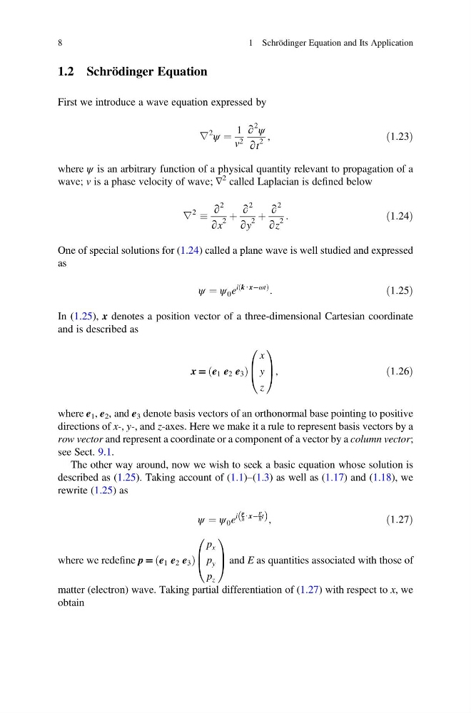
First we introduce a wave equation expressed by
∇
2 ψ ¼
1
v 2
∂
2 ψ
∂t
2
,
ð1:23Þ
where ψ is an arbitrary function of a physical quantity relevant to propagation of a
wave; v is a phase velocity of wave; ∇
2 called Laplacian is defined below
∇
2
∂
2
∂x
2
þ
∂
2
∂y
2
þ
∂
2
∂z
2
:
ð1:24Þ
One of special solutions for (1.24) called a plane wave is well studied and expressed
as
ψ ¼ ψ 0 e
i k ∙ xÀωt
ð
Þ
:
ð1:25Þ
In (1.25), x denotes a position vector of a three-dimensional Cartesian coordinate
and is described as
x = e 1 e 2 e 3
ð
Þ
x
y
z
0
B
@
1
C
A,
ð1:26Þ
where e 1 , e 2 , and e 3 denote basis vectors of an orthonormal base pointing to positive
directions of x-, y-, and z-axes. Here we make it a rule to represent basis vectors by a
row vector and represent a coordinate or a component of a vector by a column vector;
see Sect. 9.1.
The other way around, now we wish to seek a basic equation whose solution is
described as (1.25). Taking account of (1.1)–(1.3) as well as (1.17) and (1.18), we
rewrite (1.25) as
ψ ¼ ψ 0 e
i
p
ħ ∙ xÀ
E
ħ t
ð
Þ ,
ð1:27Þ
where we redefine p = e 1 e 2 e 3
ð
Þ
p x
p y
p z
0
B
@
1
C
A and E as quantities associated with those of
matter (electron) wave. Taking partial differentiation of (1.27) with respect to x, we
obtain
8
1 Schrödinger Equation and Its Application