

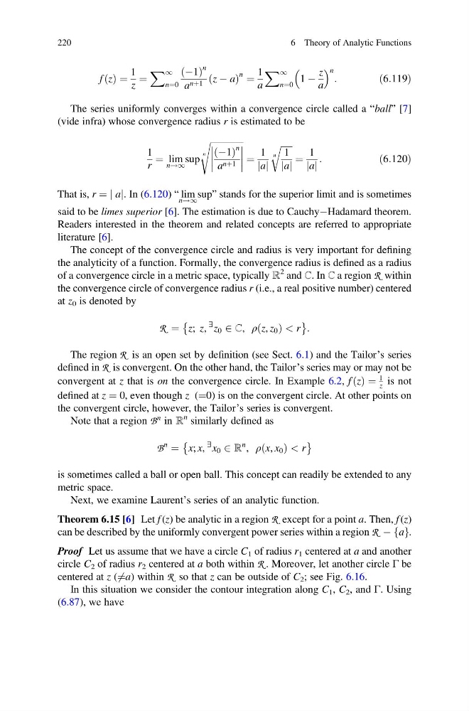
f z
ð Þ ¼
1
z
¼
X 1
n¼0
À1
ð Þ
n
a nþ1 z À a
ð
Þ
n ¼
1
a
X 1
n¼0
1 À
z
a
n :
ð6:119Þ
The series uniformly converges within a convergence circle called a “ball” [7]
(vide infra) whose convergence radius r is estimated to be
1
r
¼ lim
n!1
sup
ffiffiffiffiffiffiffiffiffiffiffiffiffiffiffi
À1
ð Þ
n
a nþ1
n
s
¼
1
a
j j
ffiffiffiffiffi ffi
1
a
j j
n
r
¼
1
a
j j
:
ð6:120Þ
That is, r ¼ j aj. In (6.120) “ lim
n!1
sup” stands for the superior limit and is sometimes
said to be limes superior [6]. The estimation is due to CauchyÀHadamard theorem.
Readers interested in the theorem and related concepts are referred to appropriate
literature [6].
The concept of the convergence circle and radius is very important for defining
the analyticity of a function. Formally, the convergence radius is defined as a radius
of a convergence circle in a metric space, typically ℝ
2 and ℂ. In ℂ a region R within
the convergence circle of convergence radius r (i.e., a real positive number) centered
at z 0 is denoted by
R ¼ z; z,
∃ z 0 2 ℂ, ρ z, z 0
ð
Þ < r
È
É :
The region R is an open set by definition (see Sect. 6.1) and the Tailor’s series
defined in R is convergent. On the other hand, the Tailor’s series may or may not be
convergent at z that is on the convergence circle. In Example 6.2, f z
ð Þ ¼
1
z is not
defined at z ¼ 0, even though z (¼0) is on the convergent circle. At other points on
the convergent circle, however, the Tailor’s series is convergent.
Note that a region B
n in ℝ
n similarly defined as
B
n
¼ x; x,
∃ x 0 2 ℝ
n , ρ x, x 0
ð
Þ < r
È
É
is sometimes called a ball or open ball. This concept can readily be extended to any
metric space.
Next, we examine Laurent’s series of an analytic function.
Theorem 6.15 [6] Let f (z) be analytic in a region R except for a point a. Then, f (z)
can be described by the uniformly convergent power series within a region R À a
f g.
Proof Let us assume that we have a circle C 1 of radius r 1 centered at a and another
circle C 2 of radius r 2 centered at a both within R . Moreover, let another circle Γ be
centered at z (6 ¼a) within R so that z can be outside of C 2 ; see Fig. 6.16.
In this situation we consider the contour integration along C 1 , C 2 , and Γ. Using
(6.87), we have
220
6 Theory of Analytic Functions
ð Þ ¼
1
z
¼
X 1
n¼0
À1
ð Þ
n
a nþ1 z À a
ð
Þ
n ¼
1
a
X 1
n¼0
1 À
z
a
n :
ð6:119Þ
The series uniformly converges within a convergence circle called a “ball” [7]
(vide infra) whose convergence radius r is estimated to be
1
r
¼ lim
n!1
sup
ffiffiffiffiffiffiffiffiffiffiffiffiffiffiffi
À1
ð Þ
n
a nþ1
n
s
¼
1
a
j j
ffiffiffiffiffi ffi
1
a
j j
n
r
¼
1
a
j j
:
ð6:120Þ
That is, r ¼ j aj. In (6.120) “ lim
n!1
sup” stands for the superior limit and is sometimes
said to be limes superior [6]. The estimation is due to CauchyÀHadamard theorem.
Readers interested in the theorem and related concepts are referred to appropriate
literature [6].
The concept of the convergence circle and radius is very important for defining
the analyticity of a function. Formally, the convergence radius is defined as a radius
of a convergence circle in a metric space, typically ℝ
2 and ℂ. In ℂ a region R within
the convergence circle of convergence radius r (i.e., a real positive number) centered
at z 0 is denoted by
R ¼ z; z,
∃ z 0 2 ℂ, ρ z, z 0
ð
Þ < r
È
É :
The region R is an open set by definition (see Sect. 6.1) and the Tailor’s series
defined in R is convergent. On the other hand, the Tailor’s series may or may not be
convergent at z that is on the convergence circle. In Example 6.2, f z
ð Þ ¼
1
z is not
defined at z ¼ 0, even though z (¼0) is on the convergent circle. At other points on
the convergent circle, however, the Tailor’s series is convergent.
Note that a region B
n in ℝ
n similarly defined as
B
n
¼ x; x,
∃ x 0 2 ℝ
n , ρ x, x 0
ð
Þ < r
È
É
is sometimes called a ball or open ball. This concept can readily be extended to any
metric space.
Next, we examine Laurent’s series of an analytic function.
Theorem 6.15 [6] Let f (z) be analytic in a region R except for a point a. Then, f (z)
can be described by the uniformly convergent power series within a region R À a
f g.
Proof Let us assume that we have a circle C 1 of radius r 1 centered at a and another
circle C 2 of radius r 2 centered at a both within R . Moreover, let another circle Γ be
centered at z (6 ¼a) within R so that z can be outside of C 2 ; see Fig. 6.16.
In this situation we consider the contour integration along C 1 , C 2 , and Γ. Using
(6.87), we have
220
6 Theory of Analytic Functions