

I
C
f z
ð Þdz ¼ 0:
ð6:84Þ
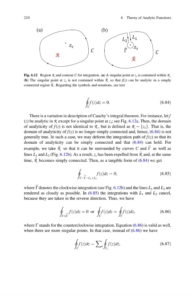
There is a variation in description of Cauchy’s integral theorem. For instance, let f
(z) be analytic in R except for a singular point at z s ; see Fig. 6.12a. Then, the domain
of analyticity of f (z) is not identical to R , but is defined as R À z s
f g. That is, the
domain of analyticity of f (z) is no longer simply connected and, hence, (6.84) is not
generally true. In such a case, we may deform the integration path of f (z) so that its
domain of analyticity can be simply connected and that (6.84) can hold. For
example, we take e
R so that it can be surrounded by curves C and e
Γ as well as
lines L 1 and L 2 (Fig. 6.12b). As a result, z s has been expelled from e
R and, at the same
time, e
R becomes simply connected. Then, as a tangible form of (6.84) we get
I
Cþ e ΓþL 1 þL 2
f z
ð Þdz ¼ 0,
ð6:85Þ
where e
Γ denotes the clockwise integration (see Fig. 6.12b) and the lines L 1 and L 2 are
rendered as closely as possible. In (6.85) the integrations with L 1 and L 2 cancel,
because they are taken in the reverse direction. Thus, we have
I
Cþ e Γ
f z
ð Þdz ¼ 0 or
I
C
f z
ð Þdz ¼
I
Γ
f z
ð Þdz,
ð6:86Þ
where Γ stands for the counterclockwise integration. Equation (6.86) is valid as well,
when there are more singular points. In that case, instead of (6.86) we have
I
C
f z
ð Þdz ¼
X
i
I
Γ i
f z
ð Þdz,
ð6:87Þ
Γ
(b)
(a)
ℛ
ℛ
Fig. 6.12 Region R and contour C for integration. (a) A singular point at z s is contained within R .
(b) The singular point at z s is not contained within e
R so that f(z) can be analytic in a simply
connected region e
R . Regarding the symbols and notations, see text
210
6 Theory of Analytic Functions
C
f z
ð Þdz ¼ 0:
ð6:84Þ
There is a variation in description of Cauchy’s integral theorem. For instance, let f
(z) be analytic in R except for a singular point at z s ; see Fig. 6.12a. Then, the domain
of analyticity of f (z) is not identical to R , but is defined as R À z s
f g. That is, the
domain of analyticity of f (z) is no longer simply connected and, hence, (6.84) is not
generally true. In such a case, we may deform the integration path of f (z) so that its
domain of analyticity can be simply connected and that (6.84) can hold. For
example, we take e
R so that it can be surrounded by curves C and e
Γ as well as
lines L 1 and L 2 (Fig. 6.12b). As a result, z s has been expelled from e
R and, at the same
time, e
R becomes simply connected. Then, as a tangible form of (6.84) we get
I
Cþ e ΓþL 1 þL 2
f z
ð Þdz ¼ 0,
ð6:85Þ
where e
Γ denotes the clockwise integration (see Fig. 6.12b) and the lines L 1 and L 2 are
rendered as closely as possible. In (6.85) the integrations with L 1 and L 2 cancel,
because they are taken in the reverse direction. Thus, we have
I
Cþ e Γ
f z
ð Þdz ¼ 0 or
I
C
f z
ð Þdz ¼
I
Γ
f z
ð Þdz,
ð6:86Þ
where Γ stands for the counterclockwise integration. Equation (6.86) is valid as well,
when there are more singular points. In that case, instead of (6.86) we have
I
C
f z
ð Þdz ¼
X
i
I
Γ i
f z
ð Þdz,
ð6:87Þ
Γ
(b)
(a)
ℛ
ℛ
Fig. 6.12 Region R and contour C for integration. (a) A singular point at z s is contained within R .
(b) The singular point at z s is not contained within e
R so that f(z) can be analytic in a simply
connected region e
R . Regarding the symbols and notations, see text
210
6 Theory of Analytic Functions