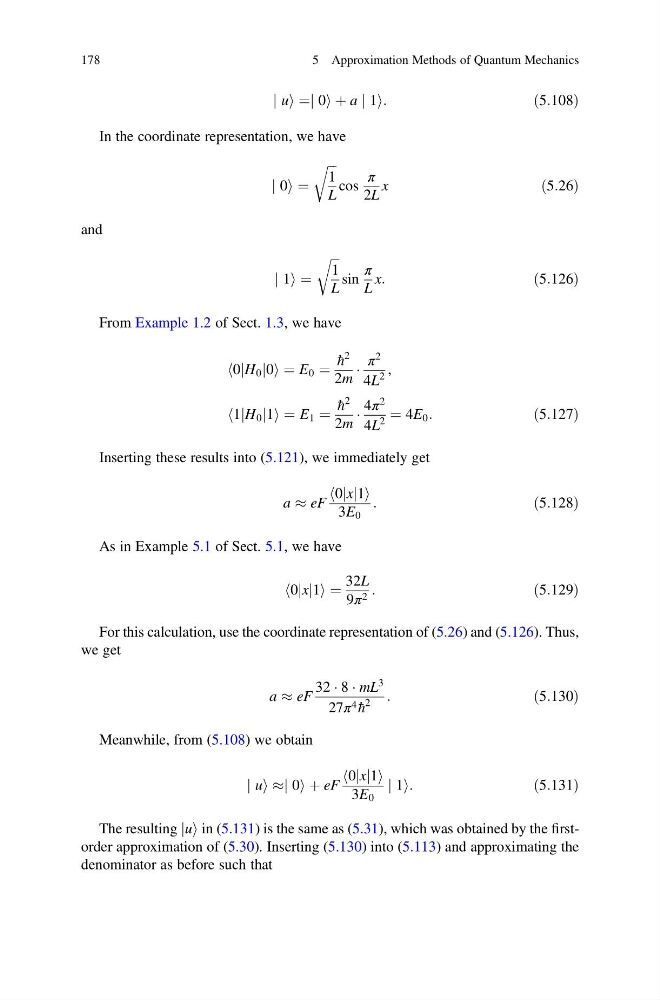
j ui ¼j 0i þ a j 1i:
ð5:108Þ
In the coordinate representation, we have
j 0i ¼
ffiffiffi
1
L
r
cos
π
2L
x
ð5:26Þ
and
j 1i ¼
ffiffiffi
1
L
r
sin
π
L
x:
ð5:126Þ
From Example 1.2 of Sect. 1.3, we have
0jH 0 j0
h
i¼ E 0 ¼
h
2
2m
Á
π
2
4L
2
,
1jH 0 j1
h
i¼ E 1 ¼
h
2
2m
Á
4π
2
4L
2
¼ 4E 0 :
ð5:127Þ
Inserting these results into (5.121), we immediately get
a % eF
0jxj1
h
i
3E 0
:
ð5:128Þ
As in Example 5.1 of Sect. 5.1, we have
0jxj1
h
i¼
32L
9π 2 :
ð5:129Þ
For this calculation, use the coordinate representation of (5.26) and (5.126). Thus,
we get
a % eF
32 Á 8 Á mL
3
27π 4 h
2
:
ð5:130Þ
Meanwhile, from (5.108) we obtain
j ui %j 0i þ eF
0jxj1
h
i
3E 0
j 1i:
ð5:131Þ
The resulting jui in (5.131) is the same as (5.31), which was obtained by the firstorder approximation of (5.30). Inserting (5.130) into (5.113) and approximating the
denominator as before such that
178
5 Approximation Methods of Quantum Mechanics