

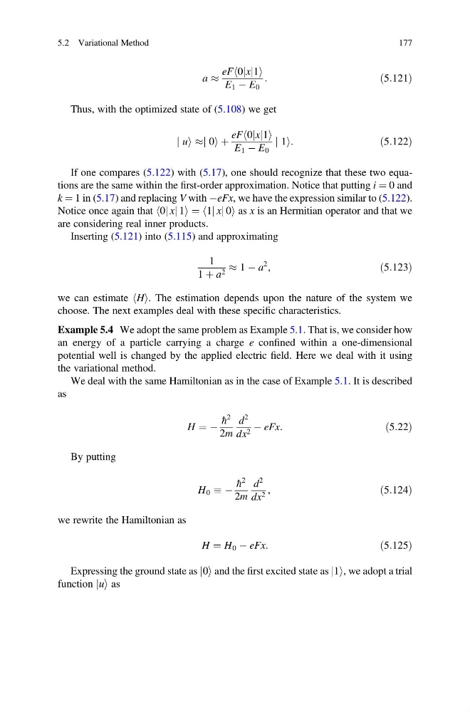
a %
eF 0jxj1
h
i
E 1 À E 0
:
ð5:121Þ
Thus, with the optimized state of (5.108) we get
j ui %j 0i þ
eF 0jxj1
h
i
E 1 À E 0
j 1i:
ð5:122Þ
If one compares (5.122) with (5.17), one should recognize that these two equations are the same within the first-order approximation. Notice that putting i ¼ 0 and
k ¼ 1 in (5.17) and replacing V with ÀeFx, we have the expression similar to (5.122).
Notice once again that h0j xj 1i ¼ h1j xj 0i as x is an Hermitian operator and that we
are considering real inner products.
Inserting (5.121) into (5.115) and approximating
1
1 þ a 2 % 1 À a
2 ,
ð5:123Þ
we can estimate hHi. The estimation depends upon the nature of the system we
choose. The next examples deal with these specific characteristics.
Example 5.4 We adopt the same problem as Example 5.1. That is, we consider how
an energy of a particle carrying a charge e confined within a one-dimensional
potential well is changed by the applied electric field. Here we deal with it using
the variational method.
We deal with the same Hamiltonian as in the case of Example 5.1. It is described
as
H ¼ À
h
2
2m
d
2
dx 2 À eFx:
ð5:22Þ
By putting
H 0 À
h
2
2m
d
2
dx 2 ,
ð5:124Þ
we rewrite the Hamiltonian as
H ¼ H 0 À eFx:
ð5:125Þ
Expressing the ground state as j0i and the first excited state as j1i, we adopt a trial
function jui as
5.2 Variational Method
177
eF 0jxj1
h
i
E 1 À E 0
:
ð5:121Þ
Thus, with the optimized state of (5.108) we get
j ui %j 0i þ
eF 0jxj1
h
i
E 1 À E 0
j 1i:
ð5:122Þ
If one compares (5.122) with (5.17), one should recognize that these two equations are the same within the first-order approximation. Notice that putting i ¼ 0 and
k ¼ 1 in (5.17) and replacing V with ÀeFx, we have the expression similar to (5.122).
Notice once again that h0j xj 1i ¼ h1j xj 0i as x is an Hermitian operator and that we
are considering real inner products.
Inserting (5.121) into (5.115) and approximating
1
1 þ a 2 % 1 À a
2 ,
ð5:123Þ
we can estimate hHi. The estimation depends upon the nature of the system we
choose. The next examples deal with these specific characteristics.
Example 5.4 We adopt the same problem as Example 5.1. That is, we consider how
an energy of a particle carrying a charge e confined within a one-dimensional
potential well is changed by the applied electric field. Here we deal with it using
the variational method.
We deal with the same Hamiltonian as in the case of Example 5.1. It is described
as
H ¼ À
h
2
2m
d
2
dx 2 À eFx:
ð5:22Þ
By putting
H 0 À
h
2
2m
d
2
dx 2 ,
ð5:124Þ
we rewrite the Hamiltonian as
H ¼ H 0 À eFx:
ð5:125Þ
Expressing the ground state as j0i and the first excited state as j1i, we adopt a trial
function jui as
5.2 Variational Method
177