

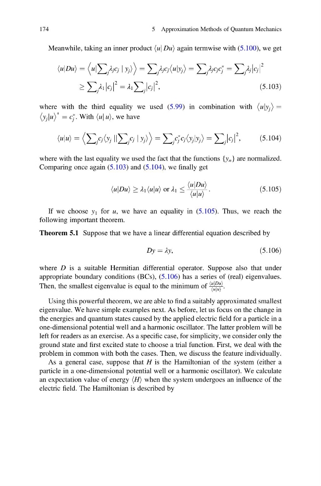
Meanwhile, taking an inner product huj Dui again termwise with (5.100), we get
ujDu
h
i¼ uj
X
j
λ j c j j y j i
D
E
¼
X
j
λ j c j ujy j
¼
X
j
λ j c j c
Ã
j ¼
X
j
λ j c j
2
!
X
j
λ 1 c j
2 ¼ λ 1
X
j
c j
2 ,
ð5:103Þ
where with the third equality we used (5.99) in combination with ujy j
¼
y j ju
à ¼ c
Ã
j . With huj ui, we have
uju
h i ¼
X
j
c j y j
jj
X
j
c j j y j i
D
E
¼
X
j
c
Ã
j c j y j jy j
¼
X
j
c j
2 ,
ð5:104Þ
where with the last equality we used the fact that the functions {y n } are normalized.
Comparing once again (5.103) and (5.104), we finally get
ujDu
h
i! λ 1 uju
h i or λ 1
ujDu
h
i
uju
h i
:
ð5:105Þ
If we choose y 1 for u, we have an equality in (5.105). Thus, we reach the
following important theorem.
Theorem 5.1 Suppose that we have a linear differential equation described by
Dy ¼ λy,
ð5:106Þ
where D is a suitable Hermitian differential operator. Suppose also that under
appropriate boundary conditions (BCs), (5.106) has a series of (real) eigenvalues.
Then, the smallest eigenvalue is equal to the minimum of
ujDu
h
i
uju
h i .
Using this powerful theorem, we are able to find a suitably approximated smallest
eigenvalue. We have simple examples next. As before, let us focus on the change in
the energies and quantum states caused by the applied electric field for a particle in a
one-dimensional potential well and a harmonic oscillator. The latter problem will be
left for readers as an exercise. As a specific case, for simplicity, we consider only the
ground state and first excited state to choose a trial function. First, we deal with the
problem in common with both the cases. Then, we discuss the feature individually.
As a general case, suppose that H is the Hamiltonian of the system (either a
particle in a one-dimensional potential well or a harmonic oscillator). We calculate
an expectation value of energy hHi when the system undergoes an influence of the
electric field. The Hamiltonian is described by
174
5 Approximation Methods of Quantum Mechanics
ujDu
h
i¼ uj
X
j
λ j c j j y j i
D
E
¼
X
j
λ j c j ujy j
¼
X
j
λ j c j c
Ã
j ¼
X
j
λ j c j
2
!
X
j
λ 1 c j
2 ¼ λ 1
X
j
c j
2 ,
ð5:103Þ
where with the third equality we used (5.99) in combination with ujy j
¼
y j ju
à ¼ c
Ã
j . With huj ui, we have
uju
h i ¼
X
j
c j y j
jj
X
j
c j j y j i
D
E
¼
X
j
c
Ã
j c j y j jy j
¼
X
j
c j
2 ,
ð5:104Þ
where with the last equality we used the fact that the functions {y n } are normalized.
Comparing once again (5.103) and (5.104), we finally get
ujDu
h
i! λ 1 uju
h i or λ 1
ujDu
h
i
uju
h i
:
ð5:105Þ
If we choose y 1 for u, we have an equality in (5.105). Thus, we reach the
following important theorem.
Theorem 5.1 Suppose that we have a linear differential equation described by
Dy ¼ λy,
ð5:106Þ
where D is a suitable Hermitian differential operator. Suppose also that under
appropriate boundary conditions (BCs), (5.106) has a series of (real) eigenvalues.
Then, the smallest eigenvalue is equal to the minimum of
ujDu
h
i
uju
h i .
Using this powerful theorem, we are able to find a suitably approximated smallest
eigenvalue. We have simple examples next. As before, let us focus on the change in
the energies and quantum states caused by the applied electric field for a particle in a
one-dimensional potential well and a harmonic oscillator. The latter problem will be
left for readers as an exercise. As a specific case, for simplicity, we consider only the
ground state and first excited state to choose a trial function. First, we deal with the
problem in common with both the cases. Then, we discuss the feature individually.
As a general case, suppose that H is the Hamiltonian of the system (either a
particle in a one-dimensional potential well or a harmonic oscillator). We calculate
an expectation value of energy hHi when the system undergoes an influence of the
electric field. The Hamiltonian is described by
174
5 Approximation Methods of Quantum Mechanics