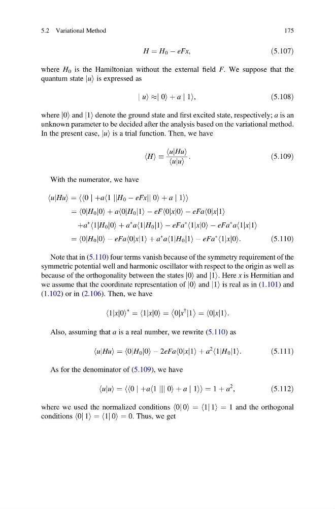
H ¼ H 0 À eFx,
ð5:107Þ
where H 0 is the Hamiltonian without the external field F. We suppose that the
quantum state jui is expressed as
j ui %j 0i þ a j 1i,
ð5:108Þ
where j0i and j1i denote the ground state and first excited state, respectively; a is an
unknown parameter to be decided after the analysis based on the variational method.
In the present case, jui is a trial function. Then, we have
H
h i
ujHu
h
i
uju
h i
:
ð5:109Þ
With the numerator, we have
ujHu
h
i¼ 0
h j þa 1
h jjH 0 À eFxjj 0i þ a j 1i
h
i
¼ 0jH 0 j0
h
iþ a 0jH 0 j1
h
iÀ eF 0jxj0
h
iÀ eFa 0jxj1
h
i
þa
à 1jH 0 j0
h
iþ a
à a 1jH 0 j1
h
iÀ eFa
à 1jxj0
h
iÀ eFa
à a 1jxj1
h
i
¼ 0jH 0 j0
h
iÀ eFa 0jxj1
h
iþ a
à a 1jH 0 j1
h
iÀ eFa
à 1jxj0
h
i:
ð5:110Þ
Note that in (5.110) four terms vanish because of the symmetry requirement of the
symmetric potential well and harmonic oscillator with respect to the origin as well as
because of the orthogonality between the states j0i and j1i. Here x is Hermitian and
we assume that the coordinate representation of j0i and j1i is real as in (1.101) and
(1.102) or in (2.106). Then, we have
1jxj0
h
i
à ¼ 1jxj0
h
i¼ 0jx
{
j1
¼ 0jxj1
h
i:
Also, assuming that a is a real number, we rewrite (5.110) as
ujHu
h
i¼ 0jH 0 j0
h
iÀ 2eFa 0jxj1
h
iþ a
2 1jH 0 j1
h
i:
ð5:111Þ
As for the denominator of (5.109), we have
uju
h i ¼ 0
h j þa 1
h jjj 0i þ a j 1i
h
i ¼ 1 þ a
2 ,
ð5:112Þ
where we used the normalized conditions h0j 0i ¼ h1j 1i ¼ 1 and the orthogonal
conditions h0j 1i ¼ h1j 0i ¼ 0. Thus, we get
5.2 Variational Method
175