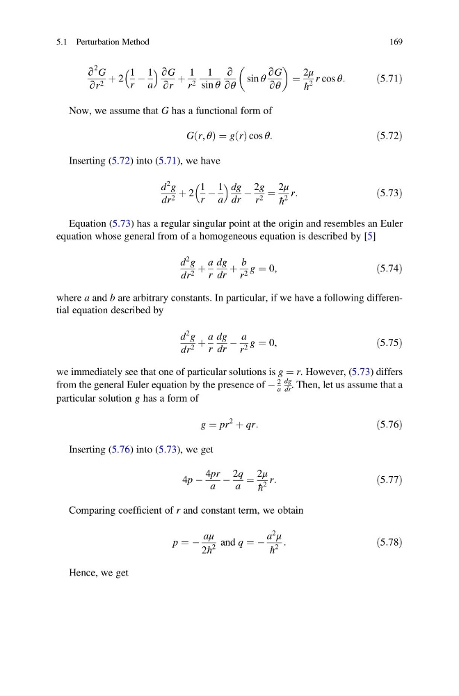
∂
2 G
∂r 2 þ 2
1
r
À
1
a
∂G
∂r
þ
1
r 2
1
sin θ
∂
∂θ
sin θ
∂G
∂θ
¼
2μ
h
2
r cos θ:
ð5:71Þ
Now, we assume that G has a functional form of
G r, θ
ð Þ ¼ g r
ð Þ cos θ:
ð5:72Þ
Inserting (5.72) into (5.71), we have
d
2 g
dr 2 þ 2
1
r
À
1
a
dg
dr
À
2g
r 2 ¼
2μ
h
2
r:
ð5:73Þ
Equation (5.73) has a regular singular point at the origin and resembles an Euler
equation whose general from of a homogeneous equation is described by [5]
d
2 g
dr 2 þ
a
r
dg
dr
þ
b
r 2 g ¼ 0,
ð5:74Þ
where a and b are arbitrary constants. In particular, if we have a following differential equation described by
d
2 g
dr 2 þ
a
r
dg
dr
À
a
r 2 g ¼ 0,
ð5:75Þ
we immediately see that one of particular solutions is g ¼ r. However, (5.73) differs
from the general Euler equation by the presence of À
2
a
dg
dr . Then, let us assume that a
particular solution g has a form of
g ¼ pr
2
þ qr:
ð5:76Þ
Inserting (5.76) into (5.73), we get
4p À
4pr
a
À
2q
a
¼
2μ
h
2
r:
ð5:77Þ
Comparing coefficient of r and constant term, we obtain
p ¼ À
aμ
2h
2
and q ¼ À
a
2
μ
h
2
:
ð5:78Þ
Hence, we get
5.1 Perturbation Method
169