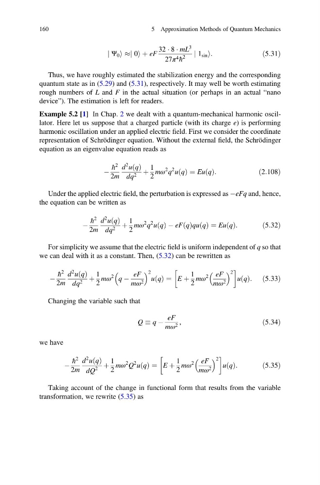
j Ψ 0 i %j 0i þ eF
32 Á 8 Á mL
3
27π 4 h
2
j 1 sin i:
ð5:31Þ
Thus, we have roughly estimated the stabilization energy and the corresponding
quantum state as in (5.29) and (5.31), respectively. It may well be worth estimating
rough numbers of L and F in the actual situation (or perhaps in an actual “nano
device”). The estimation is left for readers.
Example 5.2 [1] In Chap. 2 we dealt with a quantum-mechanical harmonic oscillator. Here let us suppose that a charged particle (with its charge e) is performing
harmonic oscillation under an applied electric field. First we consider the coordinate
representation of Schrödinger equation. Without the external field, the Schrödinger
equation as an eigenvalue equation reads as
À
h
2
2m
d
2 u q
ð Þ
dq 2 þ
1
2
mω
2 q
2 u q
ð Þ ¼ Eu q
ð Þ:
ð2:108Þ
Under the applied electric field, the perturbation is expressed as ÀeFq and, hence,
the equation can be written as
À
h
2
2m
d
2 u q
ð Þ
dq 2 þ
1
2
mω
2 q
2 u q
ð Þ À eF q
ð Þqu q
ð Þ ¼ Eu q
ð Þ:
ð5:32Þ
For simplicity we assume that the electric field is uniform independent of q so that
we can deal with it as a constant. Then, (5.32) can be rewritten as
À
h
2
2m
d
2 u q
ð Þ
dq 2 þ
1
2
mω
2 q À
eF
mω 2
2
u q
ð Þ ¼ E þ
1
2
mω
2 eF
mω 2
2 !
u q
ð Þ: ð5:33Þ
Changing the variable such that
Q q À
eF
mω 2 ,
ð5:34Þ
we have
À
h
2
2m
d
2 u q
ð Þ
dQ
2
þ
1
2
mω
2 Q
2 u q
ð Þ ¼ E þ
1
2
mω
2 eF
mω 2
2 !
u q
ð Þ:
ð5:35Þ
Taking account of the change in functional form that results from the variable
transformation, we rewrite (5.35) as
160
5 Approximation Methods of Quantum Mechanics