

M
À
ð Þ
h
i 2
&
'
kj
¼
X
p
a k δ kþ1,p a p δ pþ1,j ¼ a k a kþ1 δ kþ2,j
¼
ffiffiffiffiffiffiffiffiffiffiffiffiffiffiffiffiffiffiffiffiffiffiffiffiffiffiffiffiffi ffi
2l À k þ 1
ð
ÞÁk
p
ffiffiffiffiffiffiffiffiffiffiffiffiffiffiffiffiffiffiffiffiffiffiffiffiffiffiffiffiffiffiffiffiffiffiffiffiffiffiffiffiffiffiffiffiffiffiffiffiffiffiffiffi ffi
2l À k þ 1
ð
Þþ1
½
Ák þ 1
ð
Þ
p
δ kþ2,j , ð3:161Þ
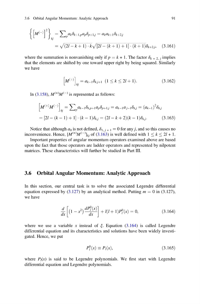
where the summation is nonvanishing only if p ¼ k + 1. The factor δ k + 2, j implies
that the elements are shifted by one toward upper right by being squared. Similarly
we have
M
þ
ð Þ
h
i
kj
¼ a kÀ1 δ k,jþ1 1 k 2l þ 1
ð
Þ :
ð3:162Þ
In (3.158), M
(+) M
(À) is represented as follows:
M
þ
ð Þ M
À
ð Þ
h
i
kj
¼
X
p
a kÀ1 δ k,pþ1 a p δ pþ1,j ¼ a kÀ1 a jÀ1 δ k,j ¼ a kÀ1
ð
Þ
2 δ k,j
¼ 2l À k À 1
ð
Þþ1
½
Ák À 1
ð
Þδ k,j ¼ 2l À k þ 2
ð
Þk À 1
ð
Þδ k,j :
ð3:163Þ
Notice that although a 0 is not defined, δ 1, j + 1 ¼ 0 for any j, and so this causes no
inconvenience. Hence, [M
(+) M
(À) ] kj of (3.163) is well defined with 1 k 2l + 1.
Important properties of angular momentum operators examined above are based
upon the fact that those operators are ladder operators and represented by nilpotent
matrices. These characteristics will further be studied in Part III.
3.6 Orbital Angular Momentum: Analytic Approach
In this section, our central task is to solve the associated Legendre differential
equation expressed by (3.127) by an analytical method. Putting m ¼ 0 in (3.127),
we have
d
dx
1 À x
2
À
Á dP
0
l x
ð Þ
dx
!
þ l l þ 1
ð
ÞP
0
l x
ð Þ ¼ 0,
ð3:164Þ
where we use a variable x instead of ξ. Equation (3.164) is called Legendre
differential equation and its characteristics and solutions have been widely investigated. Hence, we put
P
0
l x
ð Þ P l x
ð Þ,
ð3:165Þ
where P l (x) is said to be Legendre polynomials. We first start with Legendre
differential equation and Legendre polynomials.
3.6 Orbital Angular Momentum: Analytic Approach
91
À
ð Þ
h
i 2
&
'
kj
¼
X
p
a k δ kþ1,p a p δ pþ1,j ¼ a k a kþ1 δ kþ2,j
¼
ffiffiffiffiffiffiffiffiffiffiffiffiffiffiffiffiffiffiffiffiffiffiffiffiffiffiffiffiffi ffi
2l À k þ 1
ð
ÞÁk
p
ffiffiffiffiffiffiffiffiffiffiffiffiffiffiffiffiffiffiffiffiffiffiffiffiffiffiffiffiffiffiffiffiffiffiffiffiffiffiffiffiffiffiffiffiffiffiffiffiffiffiffiffi ffi
2l À k þ 1
ð
Þþ1
½
Ák þ 1
ð
Þ
p
δ kþ2,j , ð3:161Þ
where the summation is nonvanishing only if p ¼ k + 1. The factor δ k + 2, j implies
that the elements are shifted by one toward upper right by being squared. Similarly
we have
M
þ
ð Þ
h
i
kj
¼ a kÀ1 δ k,jþ1 1 k 2l þ 1
ð
Þ :
ð3:162Þ
In (3.158), M
(+) M
(À) is represented as follows:
M
þ
ð Þ M
À
ð Þ
h
i
kj
¼
X
p
a kÀ1 δ k,pþ1 a p δ pþ1,j ¼ a kÀ1 a jÀ1 δ k,j ¼ a kÀ1
ð
Þ
2 δ k,j
¼ 2l À k À 1
ð
Þþ1
½
Ák À 1
ð
Þδ k,j ¼ 2l À k þ 2
ð
Þk À 1
ð
Þδ k,j :
ð3:163Þ
Notice that although a 0 is not defined, δ 1, j + 1 ¼ 0 for any j, and so this causes no
inconvenience. Hence, [M
(+) M
(À) ] kj of (3.163) is well defined with 1 k 2l + 1.
Important properties of angular momentum operators examined above are based
upon the fact that those operators are ladder operators and represented by nilpotent
matrices. These characteristics will further be studied in Part III.
3.6 Orbital Angular Momentum: Analytic Approach
In this section, our central task is to solve the associated Legendre differential
equation expressed by (3.127) by an analytical method. Putting m ¼ 0 in (3.127),
we have
d
dx
1 À x
2
À
Á dP
0
l x
ð Þ
dx
!
þ l l þ 1
ð
ÞP
0
l x
ð Þ ¼ 0,
ð3:164Þ
where we use a variable x instead of ξ. Equation (3.164) is called Legendre
differential equation and its characteristics and solutions have been widely investigated. Hence, we put
P
0
l x
ð Þ P l x
ð Þ,
ð3:165Þ
where P l (x) is said to be Legendre polynomials. We first start with Legendre
differential equation and Legendre polynomials.
3.6 Orbital Angular Momentum: Analytic Approach
91