

M
þ
ð Þ
jl, mi ¼
ffiffiffiffiffiffiffiffiffiffiffiffiffiffiffiffiffiffiffiffiffiffiffiffiffiffiffiffiffi ffi
2l À k þ 1
ð
ÞÁk
p
jl, m þ 1i
¼
ffiffiffiffiffiffiffiffiffiffiffiffiffiffiffiffiffiffiffiffiffiffiffiffiffiffiffiffiffiffiffiffiffiffiffiffiffi
l À m
ð
Þ l þ m þ 1
ð
Þ
p
jl, m þ 1i:
ð3:157Þ
From (3.32) we have
M
2
¼ M
þ
ð Þ M
À
ð Þ
þ M z
2
À M z :
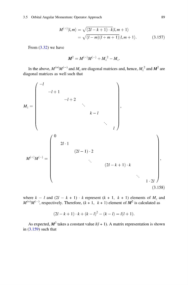
In the above, M
(+) M
(À) and M z are diagonal matrices and, hence, M z
2 and M
2 are
diagonal matrices as well such that
M z ¼
Àl
Àl þ 1
Àl þ 2
⋱
k À l
⋱
l
0
B
B
B
B
B
B
B
B
B
B
B
B
B
@
1
C
C
C
C
C
C
C
C
C
C
C
C
C
A
,
M
þ
ð Þ M
À
ð Þ
¼
0
2l Á 1
2l À 1
ð
ÞÁ2
⋱
2l À k þ 1
ð
ÞÁk
⋱
1 Á 2l
0
B
B
B
B
B
B
B
B
B
B
B
B
B
@
1
C
C
C
C
C
C
C
C
C
C
C
C
C
A
,
ð3:158Þ
where k À l and (2l À k + 1) Á k represent (k + 1, k + 1) elements of M z and
M
(+) M
(À)
, respectively. Therefore, (k + 1, k + 1) element of M
2 is calculated as
2l À k þ 1
ð
ÞÁk þ k À l
ð
Þ
2 À k À l
ð
Þ¼l l þ 1
ð
Þ:
As expected, M
2 takes a constant value l(l + 1). A matrix representation is shown
in (3.159) such that
3.5 Orbital Angular Momentum: Operator Approach
89
þ
ð Þ
jl, mi ¼
ffiffiffiffiffiffiffiffiffiffiffiffiffiffiffiffiffiffiffiffiffiffiffiffiffiffiffiffiffi ffi
2l À k þ 1
ð
ÞÁk
p
jl, m þ 1i
¼
ffiffiffiffiffiffiffiffiffiffiffiffiffiffiffiffiffiffiffiffiffiffiffiffiffiffiffiffiffiffiffiffiffiffiffiffiffi
l À m
ð
Þ l þ m þ 1
ð
Þ
p
jl, m þ 1i:
ð3:157Þ
From (3.32) we have
M
2
¼ M
þ
ð Þ M
À
ð Þ
þ M z
2
À M z :
In the above, M
(+) M
(À) and M z are diagonal matrices and, hence, M z
2 and M
2 are
diagonal matrices as well such that
M z ¼
Àl
Àl þ 1
Àl þ 2
⋱
k À l
⋱
l
0
B
B
B
B
B
B
B
B
B
B
B
B
B
@
1
C
C
C
C
C
C
C
C
C
C
C
C
C
A
,
M
þ
ð Þ M
À
ð Þ
¼
0
2l Á 1
2l À 1
ð
ÞÁ2
⋱
2l À k þ 1
ð
ÞÁk
⋱
1 Á 2l
0
B
B
B
B
B
B
B
B
B
B
B
B
B
@
1
C
C
C
C
C
C
C
C
C
C
C
C
C
A
,
ð3:158Þ
where k À l and (2l À k + 1) Á k represent (k + 1, k + 1) elements of M z and
M
(+) M
(À)
, respectively. Therefore, (k + 1, k + 1) element of M
2 is calculated as
2l À k þ 1
ð
ÞÁk þ k À l
ð
Þ
2 À k À l
ð
Þ¼l l þ 1
ð
Þ:
As expected, M
2 takes a constant value l(l + 1). A matrix representation is shown
in (3.159) such that
3.5 Orbital Angular Momentum: Operator Approach
89