

9.8 Correlated Least Squares
251
is
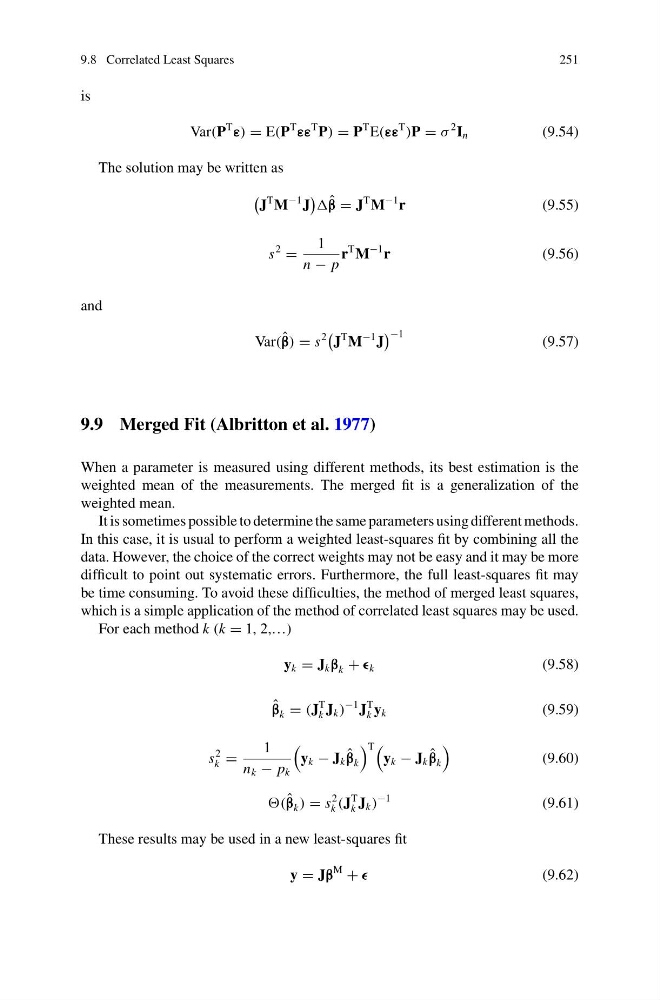
Var(P
T
ε) = E(P
T
εε
T P) = P
T E(εε
T
)P = σ
2 I n
(9.54)
The solution may be written as
J
T M
−1 J
ˆ
β = J
T M
−1 r
(9.55)
s
2
=
1
n − p
r
T M
−1 r
(9.56)
and
Var( ˆ
β) = s
2
J
T M
−1 J
−1
(9.57)
9.9 Merged Fit (Albritton et al. 1977)
When a parameter is measured using different methods, its best estimation is the
weighted mean of the measurements. The merged fit is a generalization of the
weighted mean.
It is sometimes possible to determine the same parameters using different methods.
In this case, it is usual to perform a weighted least-squares fit by combining all the
data. However, the choice of the correct weights may not be easy and it may be more
difficult to point out systematic errors. Furthermore, the full least-squares fit may
be time consuming. To avoid these difficulties, the method of merged least squares,
which is a simple application of the method of correlated least squares may be used.
For each method k (k = 1, 2,…)
y k = J k β k + k
(9.58)
ˆ
β k = (J
T
k J k )
−1 J
T
k y k
(9.59)
s
2
k =
1
n k − p k
y k − J k ˆ
β k
T
y k − J k ˆ
β k
(9.60)
( ˆ
β k ) = s
2
k (J
T
k J k )
−1
(9.61)
These results may be used in a new least-squares fit
y = Jβ
M
+
(9.62)
251
is
Var(P
T
ε) = E(P
T
εε
T P) = P
T E(εε
T
)P = σ
2 I n
(9.54)
The solution may be written as
J
T M
−1 J
ˆ
β = J
T M
−1 r
(9.55)
s
2
=
1
n − p
r
T M
−1 r
(9.56)
and
Var( ˆ
β) = s
2
J
T M
−1 J
−1
(9.57)
9.9 Merged Fit (Albritton et al. 1977)
When a parameter is measured using different methods, its best estimation is the
weighted mean of the measurements. The merged fit is a generalization of the
weighted mean.
It is sometimes possible to determine the same parameters using different methods.
In this case, it is usual to perform a weighted least-squares fit by combining all the
data. However, the choice of the correct weights may not be easy and it may be more
difficult to point out systematic errors. Furthermore, the full least-squares fit may
be time consuming. To avoid these difficulties, the method of merged least squares,
which is a simple application of the method of correlated least squares may be used.
For each method k (k = 1, 2,…)
y k = J k β k + k
(9.58)
ˆ
β k = (J
T
k J k )
−1 J
T
k y k
(9.59)
s
2
k =
1
n k − p k
y k − J k ˆ
β k
T
y k − J k ˆ
β k
(9.60)
( ˆ
β k ) = s
2
k (J
T
k J k )
−1
(9.61)
These results may be used in a new least-squares fit
y = Jβ
M
+
(9.62)