

250
9 Least-Squares Method
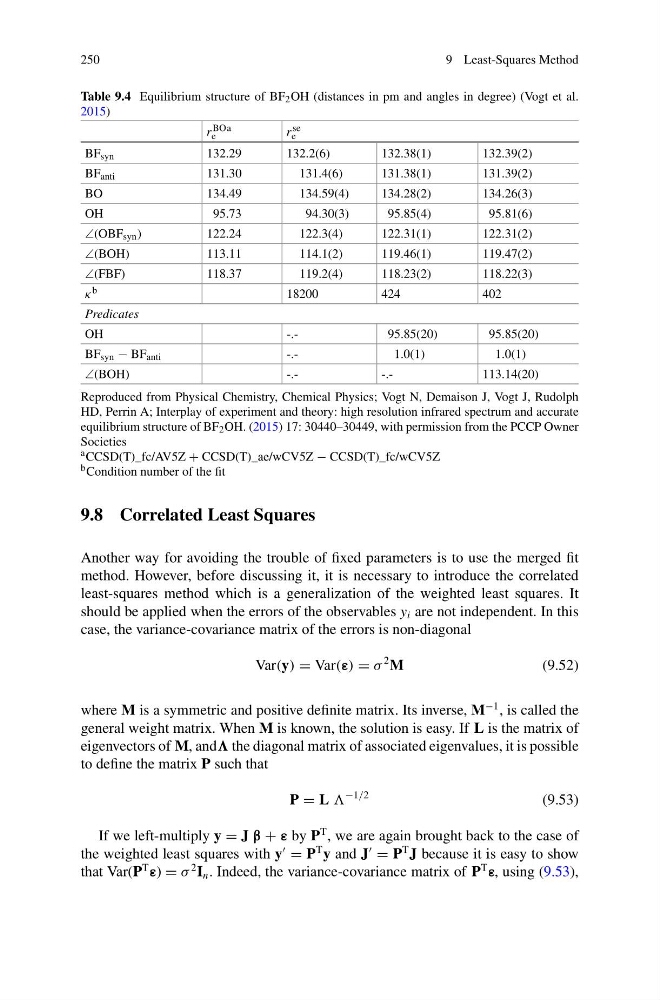
Table 9.4 Equilibrium structure of BF 2 OH (distances in pm and angles in degree) (Vogt et al.
2015)
r BO
e
a
r se
e
BF syn
132.29
132.2(6)
132.38(1)
132.39(2)
BF anti
131.30
131.4(6)
131.38(1)
131.39(2)
BO
134.49
134.59(4)
134.28(2)
134.26(3)
OH
95.73
94.30(3)
95.85(4)
95.81(6)
∠(OBF syn )
122.24
122.3(4)
122.31(1)
122.31(2)
∠(BOH)
113.11
114.1(2)
119.46(1)
119.47(2)
∠(FBF)
118.37
119.2(4)
118.23(2)
118.22(3)
κ b
18200
424
402
Predicates
OH
-.95.85(20)
95.85(20)
BF syn − BF anti
-.1.0(1)
1.0(1)
∠(BOH)
-.113.14(20)
Reproduced from Physical Chemistry, Chemical Physics; Vogt N, Demaison J, Vogt J, Rudolph
HD, Perrin A; Interplay of experiment and theory: high resolution infrared spectrum and accurate
equilibrium structure of BF 2 OH. (2015) 17: 30440–30449, with permission from the PCCP Owner
Societies
a CCSD(T)_fc/AV5Z + CCSD(T)_ae/wCV5Z − CCSD(T)_fc/wCV5Z
b Condition number of the fit
9.8 Correlated Least Squares
Another way for avoiding the trouble of fixed parameters is to use the merged fit
method. However, before discussing it, it is necessary to introduce the correlated
least-squares method which is a generalization of the weighted least squares. It
should be applied when the errors of the observables y i are not independent. In this
case, the variance-covariance matrix of the errors is non-diagonal
Var(y) = Var(ε) = σ
2 M
(9.52)
where M is a symmetric and positive definite matrix. Its inverse, M
−1 , is called the
general weight matrix. When M is known, the solution is easy. If L is the matrix of
eigenvectors of M, and the diagonal matrix of associated eigenvalues, it is possible
to define the matrix P such that
P = L
−1/2
(9.53)
If we left-multiply y = J β + ε by P
T , we are again brought back to the case of
the weighted least squares with y
= P
T y and J
= P
T J because it is easy to show
that Var(P
T
ε) = σ
2 I n . Indeed, the variance-covariance matrix of P
T
ε, using (9.53),
9 Least-Squares Method
Table 9.4 Equilibrium structure of BF 2 OH (distances in pm and angles in degree) (Vogt et al.
2015)
r BO
e
a
r se
e
BF syn
132.29
132.2(6)
132.38(1)
132.39(2)
BF anti
131.30
131.4(6)
131.38(1)
131.39(2)
BO
134.49
134.59(4)
134.28(2)
134.26(3)
OH
95.73
94.30(3)
95.85(4)
95.81(6)
∠(OBF syn )
122.24
122.3(4)
122.31(1)
122.31(2)
∠(BOH)
113.11
114.1(2)
119.46(1)
119.47(2)
∠(FBF)
118.37
119.2(4)
118.23(2)
118.22(3)
κ b
18200
424
402
Predicates
OH
-.95.85(20)
95.85(20)
BF syn − BF anti
-.1.0(1)
1.0(1)
∠(BOH)
-.113.14(20)
Reproduced from Physical Chemistry, Chemical Physics; Vogt N, Demaison J, Vogt J, Rudolph
HD, Perrin A; Interplay of experiment and theory: high resolution infrared spectrum and accurate
equilibrium structure of BF 2 OH. (2015) 17: 30440–30449, with permission from the PCCP Owner
Societies
a CCSD(T)_fc/AV5Z + CCSD(T)_ae/wCV5Z − CCSD(T)_fc/wCV5Z
b Condition number of the fit
9.8 Correlated Least Squares
Another way for avoiding the trouble of fixed parameters is to use the merged fit
method. However, before discussing it, it is necessary to introduce the correlated
least-squares method which is a generalization of the weighted least squares. It
should be applied when the errors of the observables y i are not independent. In this
case, the variance-covariance matrix of the errors is non-diagonal
Var(y) = Var(ε) = σ
2 M
(9.52)
where M is a symmetric and positive definite matrix. Its inverse, M
−1 , is called the
general weight matrix. When M is known, the solution is easy. If L is the matrix of
eigenvectors of M, and the diagonal matrix of associated eigenvalues, it is possible
to define the matrix P such that
P = L
−1/2
(9.53)
If we left-multiply y = J β + ε by P
T , we are again brought back to the case of
the weighted least squares with y
= P
T y and J
= P
T J because it is easy to show
that Var(P
T
ε) = σ
2 I n . Indeed, the variance-covariance matrix of P
T
ε, using (9.53),