

9.6 Effect of Fixed Parameters
247
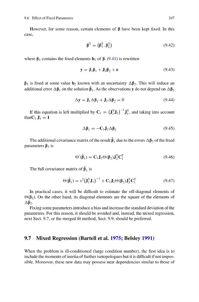
However, for some reason, certain elements of β have been kept fixed. In this
case,
β
T
=
β
T
1 , β
T
2
(9.42)
where β 2 contains the fixed elements b 2 of β. (9.41) is rewritten
y = J 1 β 1 + J 2 β 2 + ε
(9.43)
β 2 is fixed at some value b 2 known with an uncertainty β 2 . This will induce an
additional error β 1 on the solution ˆ
β 1 . As the observations y do not depend on β 2
y = J 1 β 1 + J 2 β 2 = 0
(9.44)
If this equation is left multiplied by C 1 =
J
T
1 J 1
−1 J
T
1 , and taking into account
thatC 1 J 1 = 1
β 1 = −C 1 J 2 β 2
(9.45)
The additional covariance matrix of the result ˆ
β 1 due to the errors β 2 of the fixed
parameters β 2 is
( ˆ
β 1 ) = C 1 J 2 (β 2 )J
T
2 C
T
1
(9.46)
The full covariance matrix of ˆ
β 1 is
( ˆ
β 1 ) = s
2
J
T
1 J 1
−1 + C 1 J 2 (β 2 )J
T
2 C
T
1
(9.47)
In practical cases, it will be difficult to estimate the off-diagonal elements of
(β 2 ). On the other hand, its diagonal elements are the square of the elements of
β 2 .
Fixing some parameters introduce a bias and increase the standard deviation of the
parameters. For this reason, it should be avoided and, instead, the mixed regression,
next Sect. 9.7, or the merged fit method, Sect. 9.9, should be preferred.
9.7 Mixed Regression (Bartell et al. 1975; Belsley 1991)
When the problem is ill-conditioned (large condition number), the first idea is to
include the moments of inertia of further isotopologues but it is difficult if not impossible. Moreover, these new data may possess near dependencies similar to those of
247
However, for some reason, certain elements of β have been kept fixed. In this
case,
β
T
=
β
T
1 , β
T
2
(9.42)
where β 2 contains the fixed elements b 2 of β. (9.41) is rewritten
y = J 1 β 1 + J 2 β 2 + ε
(9.43)
β 2 is fixed at some value b 2 known with an uncertainty β 2 . This will induce an
additional error β 1 on the solution ˆ
β 1 . As the observations y do not depend on β 2
y = J 1 β 1 + J 2 β 2 = 0
(9.44)
If this equation is left multiplied by C 1 =
J
T
1 J 1
−1 J
T
1 , and taking into account
thatC 1 J 1 = 1
β 1 = −C 1 J 2 β 2
(9.45)
The additional covariance matrix of the result ˆ
β 1 due to the errors β 2 of the fixed
parameters β 2 is
( ˆ
β 1 ) = C 1 J 2 (β 2 )J
T
2 C
T
1
(9.46)
The full covariance matrix of ˆ
β 1 is
( ˆ
β 1 ) = s
2
J
T
1 J 1
−1 + C 1 J 2 (β 2 )J
T
2 C
T
1
(9.47)
In practical cases, it will be difficult to estimate the off-diagonal elements of
(β 2 ). On the other hand, its diagonal elements are the square of the elements of
β 2 .
Fixing some parameters introduce a bias and increase the standard deviation of the
parameters. For this reason, it should be avoided and, instead, the mixed regression,
next Sect. 9.7, or the merged fit method, Sect. 9.9, should be preferred.
9.7 Mixed Regression (Bartell et al. 1975; Belsley 1991)
When the problem is ill-conditioned (large condition number), the first idea is to
include the moments of inertia of further isotopologues but it is difficult if not impossible. Moreover, these new data may possess near dependencies similar to those of