

246
9 Least-Squares Method
u i = |r i |/s
(9.37)
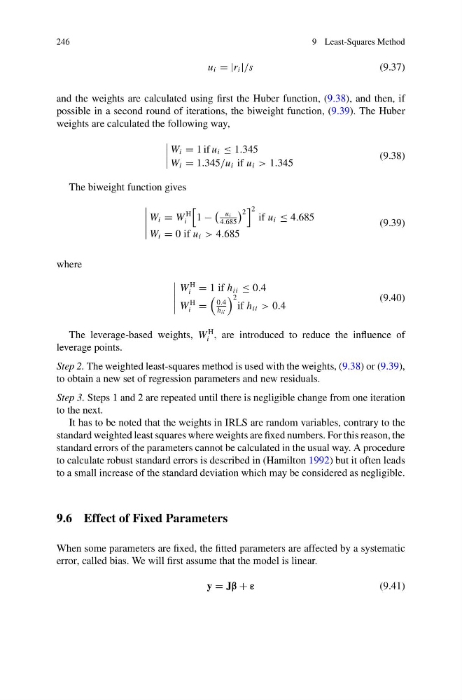
and the weights are calculated using first the Huber function, (9.38), and then, if
possible in a second round of iterations, the biweight function, (9.39). The Huber
weights are calculated the following way,
W i = 1 if u i ≤ 1.345
W i = 1.345/u i if u i > 1.345
(9.38)
The biweight function gives
W i = W
H
i
1 −
u i
4.685
2
2
if u i ≤ 4.685
W i = 0 if u i > 4.685
(9.39)
where
W
H
i = 1 if h ii ≤ 0.4
W
H
i =
0.4
h ii
2
if h ii > 0.4
(9.40)
The leverage-based weights, W
H
i , are introduced to reduce the influence of
leverage points.
Step 2. The weighted least-squares method is used with the weights, (9.38) or (9.39),
to obtain a new set of regression parameters and new residuals.
Step 3. Steps 1 and 2 are repeated until there is negligible change from one iteration
to the next.
It has to be noted that the weights in IRLS are random variables, contrary to the
standard weighted least squares where weights are fixed numbers. For this reason, the
standard errors of the parameters cannot be calculated in the usual way. A procedure
to calculate robust standard errors is described in (Hamilton 1992) but it often leads
to a small increase of the standard deviation which may be considered as negligible.
9.6 Effect of Fixed Parameters
When some parameters are fixed, the fitted parameters are affected by a systematic
error, called bias. We will first assume that the model is linear.
y = Jβ + ε
(9.41)
9 Least-Squares Method
u i = |r i |/s
(9.37)
and the weights are calculated using first the Huber function, (9.38), and then, if
possible in a second round of iterations, the biweight function, (9.39). The Huber
weights are calculated the following way,
W i = 1 if u i ≤ 1.345
W i = 1.345/u i if u i > 1.345
(9.38)
The biweight function gives
W i = W
H
i
1 −
u i
4.685
2
2
if u i ≤ 4.685
W i = 0 if u i > 4.685
(9.39)
where
W
H
i = 1 if h ii ≤ 0.4
W
H
i =
0.4
h ii
2
if h ii > 0.4
(9.40)
The leverage-based weights, W
H
i , are introduced to reduce the influence of
leverage points.
Step 2. The weighted least-squares method is used with the weights, (9.38) or (9.39),
to obtain a new set of regression parameters and new residuals.
Step 3. Steps 1 and 2 are repeated until there is negligible change from one iteration
to the next.
It has to be noted that the weights in IRLS are random variables, contrary to the
standard weighted least squares where weights are fixed numbers. For this reason, the
standard errors of the parameters cannot be calculated in the usual way. A procedure
to calculate robust standard errors is described in (Hamilton 1992) but it often leads
to a small increase of the standard deviation which may be considered as negligible.
9.6 Effect of Fixed Parameters
When some parameters are fixed, the fitted parameters are affected by a systematic
error, called bias. We will first assume that the model is linear.
y = Jβ + ε
(9.41)