

236
9 Least-Squares Method
(β) = s
2
J
T J
−1
(9.7)
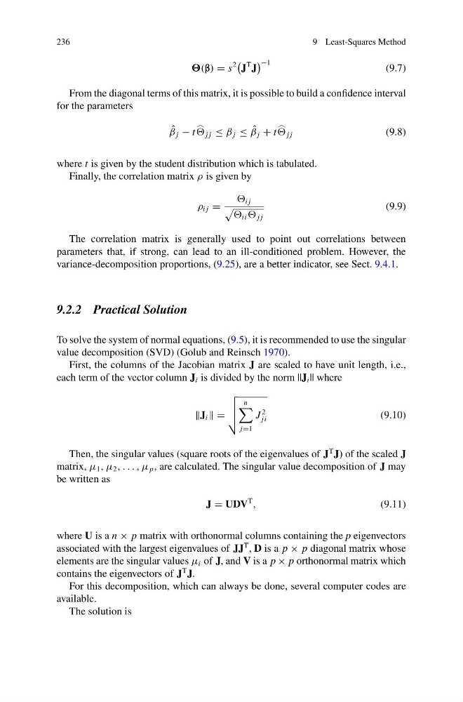
From the diagonal terms of this matrix, it is possible to build a confidence interval
for the parameters
ˆ
β j − t
j j ≤ β j ≤ ˆ
β j + t
j j
(9.8)
where t is given by the student distribution which is tabulated.
Finally, the correlation matrix ρ is given by
ρ i j =
i j
ii j j
(9.9)
The correlation matrix is generally used to point out correlations between
parameters that, if strong, can lead to an ill-conditioned problem. However, the
variance-decomposition proportions, (9.25), are a better indicator, see Sect. 9.4.1.
9.2.2 Practical Solution
To solve the system of normal equations, (9.5), it is recommended to use the singular
value decomposition (SVD) (Golub and Reinsch 1970).
First, the columns of the Jacobian matrix J are scaled to have unit length, i.e.,
each term of the vector column J i is divided by the norm ||J i || where
J i =
n
j=1
J
2
ji
(9.10)
Then, the singular values (square roots of the eigenvalues of J
T J) of the scaled J
matrix, μ 1 , μ 2 , . . . , μ p , are calculated. The singular value decomposition of J may
be written as
J = UDV
T
,
(9.11)
where U is a n × p matrix with orthonormal columns containing the p eigenvectors
associated with the largest eigenvalues of JJ
T , D is a p × p diagonal matrix whose
elements are the singular values μ i of J, and V is a p × p orthonormal matrix which
contains the eigenvectors of J
T J.
For this decomposition, which can always be done, several computer codes are
available.
The solution is
9 Least-Squares Method
(β) = s
2
J
T J
−1
(9.7)
From the diagonal terms of this matrix, it is possible to build a confidence interval
for the parameters
ˆ
β j − t
j j ≤ β j ≤ ˆ
β j + t
j j
(9.8)
where t is given by the student distribution which is tabulated.
Finally, the correlation matrix ρ is given by
ρ i j =
i j
ii j j
(9.9)
The correlation matrix is generally used to point out correlations between
parameters that, if strong, can lead to an ill-conditioned problem. However, the
variance-decomposition proportions, (9.25), are a better indicator, see Sect. 9.4.1.
9.2.2 Practical Solution
To solve the system of normal equations, (9.5), it is recommended to use the singular
value decomposition (SVD) (Golub and Reinsch 1970).
First, the columns of the Jacobian matrix J are scaled to have unit length, i.e.,
each term of the vector column J i is divided by the norm ||J i || where
J i =
n
j=1
J
2
ji
(9.10)
Then, the singular values (square roots of the eigenvalues of J
T J) of the scaled J
matrix, μ 1 , μ 2 , . . . , μ p , are calculated. The singular value decomposition of J may
be written as
J = UDV
T
,
(9.11)
where U is a n × p matrix with orthonormal columns containing the p eigenvectors
associated with the largest eigenvalues of JJ
T , D is a p × p diagonal matrix whose
elements are the singular values μ i of J, and V is a p × p orthonormal matrix which
contains the eigenvectors of J
T J.
For this decomposition, which can always be done, several computer codes are
available.
The solution is