

9.2 Nonlinear Least-Squares Method
235
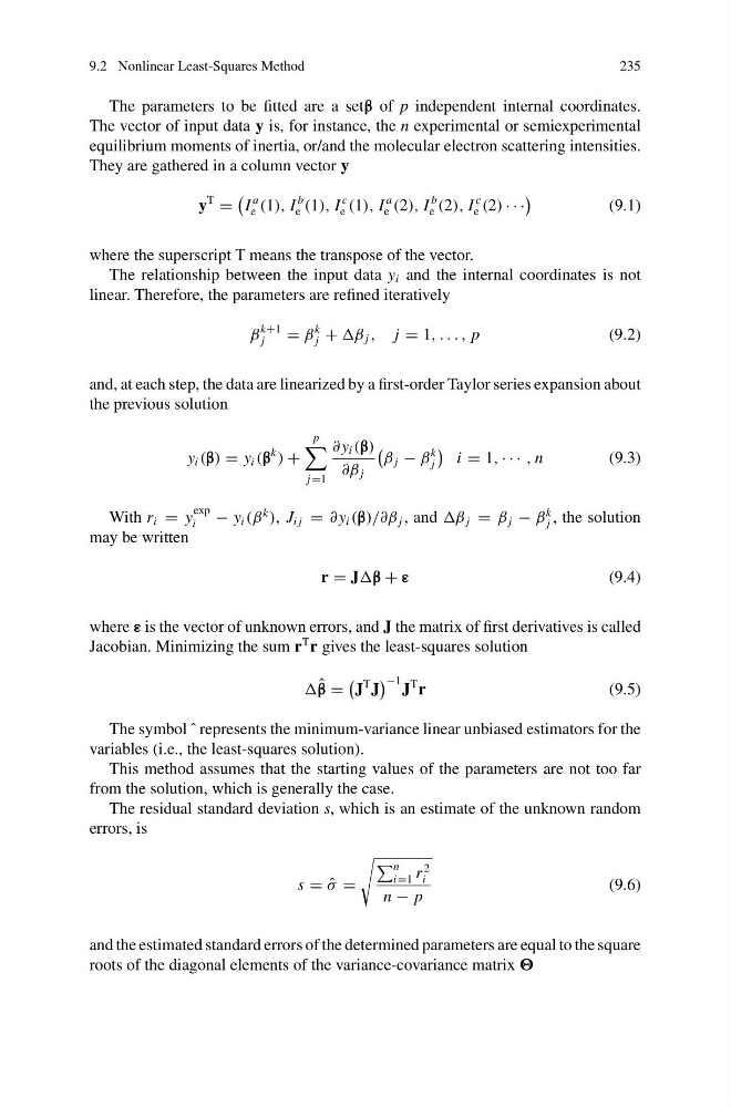
The parameters to be fitted are a setβ of p independent internal coordinates.
The vector of input data y is, for instance, the n experimental or semiexperimental
equilibrium moments of inertia, or/and the molecular electron scattering intensities.
They are gathered in a column vector y
y
T
=
I
a
e (1), I
b
e (1), I
c
e (1), I
a
e (2), I
b
e (2), I
c
e (2) · · ·
(9.1)
where the superscript T means the transpose of the vector.
The relationship between the input data y i and the internal coordinates is not
linear. Therefore, the parameters are refined iteratively
β
k+1
j
= β
k
j + β j , j = 1, . . . , p
(9.2)
and, at each step, the data are linearized by a first-order Taylor series expansion about
the previous solution
y i (β) = y i (β
k
) +
p
j=1
∂ y i (β)
∂β j
β j − β
k
j
i = 1, · · · , n
(9.3)
With r i = y
exp
i
− y i (β
k
), J i j = ∂ y i (β)/∂β j , and β j = β j − β
k
j , the solution
may be written
r = Jβ + ε
(9.4)
where ε is the vector of unknown errors, and J the matrix of first derivatives is called
Jacobian. Minimizing the sum r
T r gives the least-squares solution
ˆ
β =
J
T J
−1 J
T r
(9.5)
The symbol ˆ represents the minimum-variance linear unbiased estimators for the
variables (i.e., the least-squares solution).
This method assumes that the starting values of the parameters are not too far
from the solution, which is generally the case.
The residual standard deviation s, which is an estimate of the unknown random
errors, is
s = ˆ
σ =
n
i=1 r
2
i
n − p
(9.6)
and the estimated standard errors of the determined parameters are equal to the square
roots of the diagonal elements of the variance-covariance matrix
235
The parameters to be fitted are a setβ of p independent internal coordinates.
The vector of input data y is, for instance, the n experimental or semiexperimental
equilibrium moments of inertia, or/and the molecular electron scattering intensities.
They are gathered in a column vector y
y
T
=
I
a
e (1), I
b
e (1), I
c
e (1), I
a
e (2), I
b
e (2), I
c
e (2) · · ·
(9.1)
where the superscript T means the transpose of the vector.
The relationship between the input data y i and the internal coordinates is not
linear. Therefore, the parameters are refined iteratively
β
k+1
j
= β
k
j + β j , j = 1, . . . , p
(9.2)
and, at each step, the data are linearized by a first-order Taylor series expansion about
the previous solution
y i (β) = y i (β
k
) +
p
j=1
∂ y i (β)
∂β j
β j − β
k
j
i = 1, · · · , n
(9.3)
With r i = y
exp
i
− y i (β
k
), J i j = ∂ y i (β)/∂β j , and β j = β j − β
k
j , the solution
may be written
r = Jβ + ε
(9.4)
where ε is the vector of unknown errors, and J the matrix of first derivatives is called
Jacobian. Minimizing the sum r
T r gives the least-squares solution
ˆ
β =
J
T J
−1 J
T r
(9.5)
The symbol ˆ represents the minimum-variance linear unbiased estimators for the
variables (i.e., the least-squares solution).
This method assumes that the starting values of the parameters are not too far
from the solution, which is generally the case.
The residual standard deviation s, which is an estimate of the unknown random
errors, is
s = ˆ
σ =
n
i=1 r
2
i
n − p
(9.6)
and the estimated standard errors of the determined parameters are equal to the square
roots of the diagonal elements of the variance-covariance matrix