

9.2 Nonlinear Least-Squares Method
237
ˆ
β = VD
−1 U
T y
(9.12)
and
(β) = s
2
J
T J
−1 = s
2 VD
−2 V
T
(9.13)
i.e.,
ˆ
σ ( ˆ
β k ) = s
2
p
j
V k j
μ j
2
(9.14)
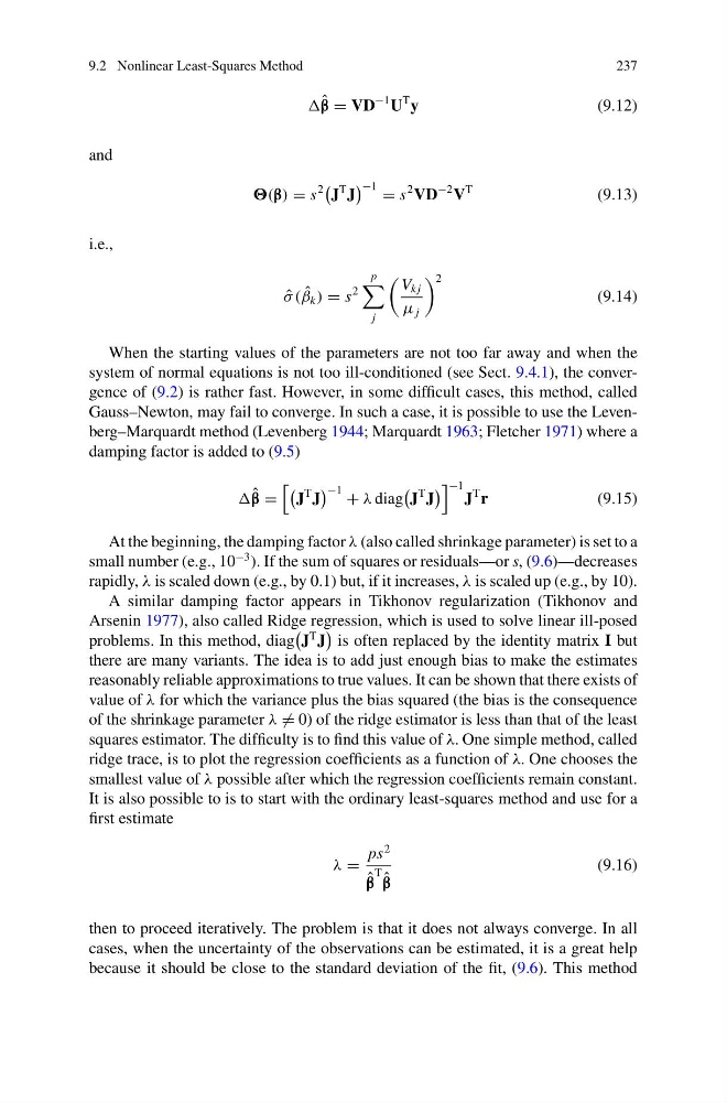
When the starting values of the parameters are not too far away and when the
system of normal equations is not too ill-conditioned (see Sect. 9.4.1), the convergence of (9.2) is rather fast. However, in some difficult cases, this method, called
Gauss–Newton, may fail to converge. In such a case, it is possible to use the Levenberg–Marquardt method (Levenberg 1944; Marquardt 1963; Fletcher 1971) where a
damping factor is added to (9.5)
ˆ
β =
J
T J
−1 + λ diag
J
T J
−1
J
T r
(9.15)
At the beginning, the damping factor λ (also called shrinkage parameter) is set to a
small number (e.g., 10
−3 ). If the sum of squares or residuals—or s, (9.6)—decreases
rapidly, λ is scaled down (e.g., by 0.1) but, if it increases, λ is scaled up (e.g., by 10).
A similar damping factor appears in Tikhonov regularization (Tikhonov and
Arsenin 1977), also called Ridge regression, which is used to solve linear ill-posed
problems. In this method, diag
J
T J
is often replaced by the identity matrix I but
there are many variants. The idea is to add just enough bias to make the estimates
reasonably reliable approximations to true values. It can be shown that there exists of
value of λ for which the variance plus the bias squared (the bias is the consequence
of the shrinkage parameter λ = 0) of the ridge estimator is less than that of the least
squares estimator. The difficulty is to find this value of λ. One simple method, called
ridge trace, is to plot the regression coefficients as a function of λ. One chooses the
smallest value of λ possible after which the regression coefficients remain constant.
It is also possible to is to start with the ordinary least-squares method and use for a
first estimate
λ =
ps
2
ˆ
β
T ˆ
β
(9.16)
then to proceed iteratively. The problem is that it does not always converge. In all
cases, when the uncertainty of the observations can be estimated, it is a great help
because it should be close to the standard deviation of the fit, (9.6). This method
237
ˆ
β = VD
−1 U
T y
(9.12)
and
(β) = s
2
J
T J
−1 = s
2 VD
−2 V
T
(9.13)
i.e.,
ˆ
σ ( ˆ
β k ) = s
2
p
j
V k j
μ j
2
(9.14)
When the starting values of the parameters are not too far away and when the
system of normal equations is not too ill-conditioned (see Sect. 9.4.1), the convergence of (9.2) is rather fast. However, in some difficult cases, this method, called
Gauss–Newton, may fail to converge. In such a case, it is possible to use the Levenberg–Marquardt method (Levenberg 1944; Marquardt 1963; Fletcher 1971) where a
damping factor is added to (9.5)
ˆ
β =
J
T J
−1 + λ diag
J
T J
−1
J
T r
(9.15)
At the beginning, the damping factor λ (also called shrinkage parameter) is set to a
small number (e.g., 10
−3 ). If the sum of squares or residuals—or s, (9.6)—decreases
rapidly, λ is scaled down (e.g., by 0.1) but, if it increases, λ is scaled up (e.g., by 10).
A similar damping factor appears in Tikhonov regularization (Tikhonov and
Arsenin 1977), also called Ridge regression, which is used to solve linear ill-posed
problems. In this method, diag
J
T J
is often replaced by the identity matrix I but
there are many variants. The idea is to add just enough bias to make the estimates
reasonably reliable approximations to true values. It can be shown that there exists of
value of λ for which the variance plus the bias squared (the bias is the consequence
of the shrinkage parameter λ = 0) of the ridge estimator is less than that of the least
squares estimator. The difficulty is to find this value of λ. One simple method, called
ridge trace, is to plot the regression coefficients as a function of λ. One chooses the
smallest value of λ possible after which the regression coefficients remain constant.
It is also possible to is to start with the ordinary least-squares method and use for a
first estimate
λ =
ps
2
ˆ
β
T ˆ
β
(9.16)
then to proceed iteratively. The problem is that it does not always converge. In all
cases, when the uncertainty of the observations can be estimated, it is a great help
because it should be close to the standard deviation of the fit, (9.6). This method