

4.8 Asymmetric Molecule
89
consequence is that the experimental rotational constants are slightly affected by the
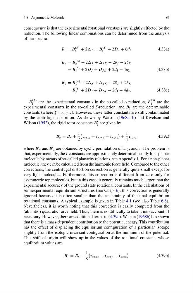
reduction. The following linear combinations can be determined from the analysis
of the spectra:
B z = B
(A)
z
+ 2 J = B
(S)
z + 2D J + 6d 2
(4.38a)
B x = B
(A)
x + 2 J + J K − 2δ J − 2δ K
= B
(S)
x + 2D J + D J K + 2d 1 + 4d 2
(4.38b)
B y = B
(A)
y + 2 J + J K + 2δ J + 2δ K
= B
(S)
y + 2D J + D J K − 2d 1 + 4d 2 .
(4.38c)
B
(A)
ξ
are the experimental constants in the so-called A-reduction, B
(S)
ξ
are the
experimental constants in the so-called S-reduction, and B ξ are the determinable
constants (where ξ = x, y, z). However, these latter constants are still contaminated
by the centrifugal distortion. As shown by Watson (1968a, b) and Kivelson and
Wilson (1952), the rigid rotor constants B
ξ are given by
B
x = B x +
1
2
τ yyzz + τ xyxy + τ xzxz
+
1
4
τ yzyz
(4.39a)
where B
y and B
z are obtained by cyclic permutation of x, y, and z. The problem is
that, experimentally, the τ constants are approximately determinable only for a planar
molecule by means of so-called planarity relations, see Appendix 1. For a non-planar
molecule, they can be calculated from the harmonic force field. Compared to the other
corrections, the centrifugal distortion correction is generally quite small except for
very light molecules. Furthermore, this correction is different from zero only for
asymmetric top molecules, but in this case, it generally remains much larger than the
experimental accuracy of the ground state rotational constants. In the calculations of
semiexperimental equilibrium structures (see Chap. 6), this correction is generally
ignored because it is often smaller than the uncertainty of the final equilibrium
rotational constants. A typical example is given in Table 4.1 (see also Table 6.8).
Nevertheless, it is worth noting that this correction is easily computed from the
(ab initio) quadratic force field. Thus, there is no difficulty to take it into account, if
necessary. However, there are additional terms to (4.39a). Watson (1968b) has shown
that there is a mass-dependent contribution to the potential energy. This contribution
has the effect of displacing the equilibrium configuration of a particular isotope
slightly from the isotopic invariant configuration at the minimum of the potential.
This shift of origin will show up in the values of the rotational constants whose
equilibrium values are
B
x = B x −
1
8
τ xxxx + τ xxyy + τ xxzz
(4.39b)
89
consequence is that the experimental rotational constants are slightly affected by the
reduction. The following linear combinations can be determined from the analysis
of the spectra:
B z = B
(A)
z
+ 2 J = B
(S)
z + 2D J + 6d 2
(4.38a)
B x = B
(A)
x + 2 J + J K − 2δ J − 2δ K
= B
(S)
x + 2D J + D J K + 2d 1 + 4d 2
(4.38b)
B y = B
(A)
y + 2 J + J K + 2δ J + 2δ K
= B
(S)
y + 2D J + D J K − 2d 1 + 4d 2 .
(4.38c)
B
(A)
ξ
are the experimental constants in the so-called A-reduction, B
(S)
ξ
are the
experimental constants in the so-called S-reduction, and B ξ are the determinable
constants (where ξ = x, y, z). However, these latter constants are still contaminated
by the centrifugal distortion. As shown by Watson (1968a, b) and Kivelson and
Wilson (1952), the rigid rotor constants B
ξ are given by
B
x = B x +
1
2
τ yyzz + τ xyxy + τ xzxz
+
1
4
τ yzyz
(4.39a)
where B
y and B
z are obtained by cyclic permutation of x, y, and z. The problem is
that, experimentally, the τ constants are approximately determinable only for a planar
molecule by means of so-called planarity relations, see Appendix 1. For a non-planar
molecule, they can be calculated from the harmonic force field. Compared to the other
corrections, the centrifugal distortion correction is generally quite small except for
very light molecules. Furthermore, this correction is different from zero only for
asymmetric top molecules, but in this case, it generally remains much larger than the
experimental accuracy of the ground state rotational constants. In the calculations of
semiexperimental equilibrium structures (see Chap. 6), this correction is generally
ignored because it is often smaller than the uncertainty of the final equilibrium
rotational constants. A typical example is given in Table 4.1 (see also Table 6.8).
Nevertheless, it is worth noting that this correction is easily computed from the
(ab initio) quadratic force field. Thus, there is no difficulty to take it into account, if
necessary. However, there are additional terms to (4.39a). Watson (1968b) has shown
that there is a mass-dependent contribution to the potential energy. This contribution
has the effect of displacing the equilibrium configuration of a particular isotope
slightly from the isotopic invariant configuration at the minimum of the potential.
This shift of origin will show up in the values of the rotational constants whose
equilibrium values are
B
x = B x −
1
8
τ xxxx + τ xxyy + τ xxzz
(4.39b)