

30
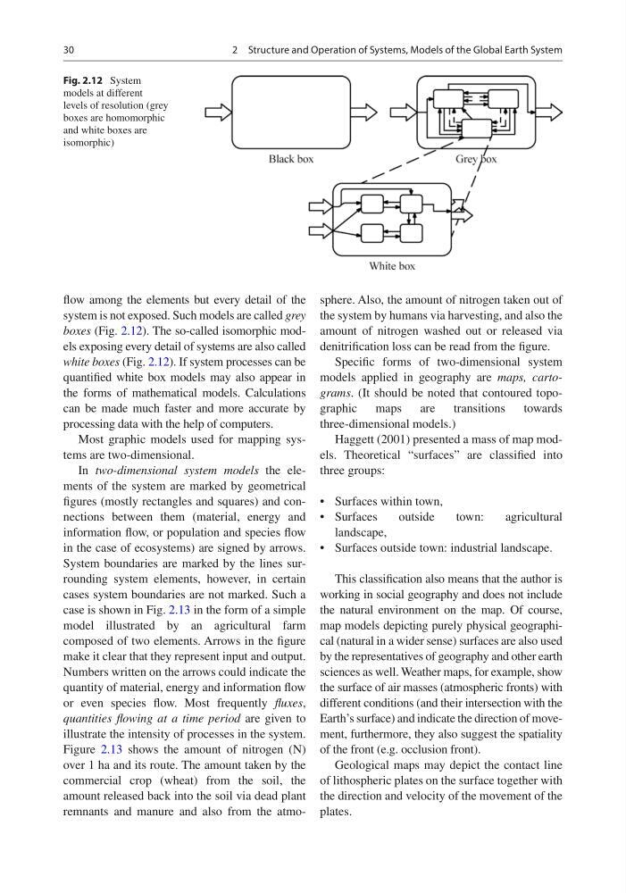
flow among the elements but every detail of the
system is not exposed. Such models are called grey
boxes (Fig. 2.12). The so-called isomorphic models exposing every detail of systems are also called
white boxes (Fig. 2.12). If system processes can be
quantified white box models may also appear in
the forms of mathematical models. Calculations
can be made much faster and more accurate by
processing data with the help of computers.
Most graphic models used for mapping systems are two-dimensional.
In two-dimensional system models the elements of the system are marked by geometrical
figures (mostly rectangles and squares) and connections between them (material, energy and
information flow, or population and species flow
in the case of ecosystems) are signed by arrows.
System boundaries are marked by the lines surrounding system elements, however, in certain
cases system boundaries are not marked. Such a
case is shown in Fig. 2.13 in the form of a simple
model illustrated by an agricultural farm
composed of two elements. Arrows in the figure
make it clear that they represent input and output.
Numbers written on the arrows could indicate the
quantity of material, energy and information flow
or even species flow. Most frequently fluxes,
quantities flowing at a time period are given to
illustrate the intensity of processes in the system.
Figure 2.13 shows the amount of nitrogen (N)
over 1 ha and its route. The amount taken by the
commercial crop (wheat) from the soil, the
amount released back into the soil via dead plant
remnants and manure and also from the atmosphere. Also, the amount of nitrogen taken out of
the system by humans via harvesting, and also the
amount of nitrogen washed out or released via
denitrification loss can be read from the figure.
Specific forms of two-dimensional system
models applied in geography are maps, cartograms. (It should be noted that contoured topographic maps are transitions towards
three-dimensional models.)
Haggett (2001) presented a mass of map models. Theoretical “surfaces” are classified into
three groups:
• Surfaces within town,
• Surfaces
outside
town:
agricultural
landscape,
• Surfaces outside town: industrial landscape.
This classification also means that the author is
working in social geography and does not include
the natural environment on the map. Of course,
map models depicting purely physical geographical (natural in a wider sense) surfaces are also used
by the representatives of geography and other earth
sciences as well. Weather maps, for example, show
the surface of air masses (atmospheric fronts) with
different conditions (and their intersection with the
Earth’s surface) and indicate the direction of movement, furthermore, they also suggest the spatiality
of the front (e.g. occlusion front).
Geological maps may depict the contact line
of lithospheric plates on the surface together with
the direction and velocity of the movement of the
plates.
Fig. 2.12 System
models at different
levels of resolution (grey
boxes are homomorphic
and white boxes are
isomorphic)
2 Structure and Operation of Systems, Models of the Global Earth System
flow among the elements but every detail of the
system is not exposed. Such models are called grey
boxes (Fig. 2.12). The so-called isomorphic models exposing every detail of systems are also called
white boxes (Fig. 2.12). If system processes can be
quantified white box models may also appear in
the forms of mathematical models. Calculations
can be made much faster and more accurate by
processing data with the help of computers.
Most graphic models used for mapping systems are two-dimensional.
In two-dimensional system models the elements of the system are marked by geometrical
figures (mostly rectangles and squares) and connections between them (material, energy and
information flow, or population and species flow
in the case of ecosystems) are signed by arrows.
System boundaries are marked by the lines surrounding system elements, however, in certain
cases system boundaries are not marked. Such a
case is shown in Fig. 2.13 in the form of a simple
model illustrated by an agricultural farm
composed of two elements. Arrows in the figure
make it clear that they represent input and output.
Numbers written on the arrows could indicate the
quantity of material, energy and information flow
or even species flow. Most frequently fluxes,
quantities flowing at a time period are given to
illustrate the intensity of processes in the system.
Figure 2.13 shows the amount of nitrogen (N)
over 1 ha and its route. The amount taken by the
commercial crop (wheat) from the soil, the
amount released back into the soil via dead plant
remnants and manure and also from the atmosphere. Also, the amount of nitrogen taken out of
the system by humans via harvesting, and also the
amount of nitrogen washed out or released via
denitrification loss can be read from the figure.
Specific forms of two-dimensional system
models applied in geography are maps, cartograms. (It should be noted that contoured topographic maps are transitions towards
three-dimensional models.)
Haggett (2001) presented a mass of map models. Theoretical “surfaces” are classified into
three groups:
• Surfaces within town,
• Surfaces
outside
town:
agricultural
landscape,
• Surfaces outside town: industrial landscape.
This classification also means that the author is
working in social geography and does not include
the natural environment on the map. Of course,
map models depicting purely physical geographical (natural in a wider sense) surfaces are also used
by the representatives of geography and other earth
sciences as well. Weather maps, for example, show
the surface of air masses (atmospheric fronts) with
different conditions (and their intersection with the
Earth’s surface) and indicate the direction of movement, furthermore, they also suggest the spatiality
of the front (e.g. occlusion front).
Geological maps may depict the contact line
of lithospheric plates on the surface together with
the direction and velocity of the movement of the
plates.
Fig. 2.12 System
models at different
levels of resolution (grey
boxes are homomorphic
and white boxes are
isomorphic)
2 Structure and Operation of Systems, Models of the Global Earth System