

A more convenient option is to use devices based on ferromagnetic susceptibility
(Vecchia et al. 2009; Strutz et al. 2016) that possess higher sensitivity and enable
realistic simulation of field conditions. The one-dimensional column device and the
cascade column with ferromagnetic susceptibility detector described in this chapter
were both developed at the Technical University of Liberec.
30.2 One-Dimensional Column Device
This device enables mobility tests in long columns where, in a single experiment, it is
possible to combine a standard assay for migration of nZVI particles in suspension with
a washing test by simply replacing the original suspension with nanoparticle-free water.
For one-dimensional experimental arrangement, the basis of the device is a short
length coil, freely encircling a column with the possibility of defined shifting in the
direction of the axis of the column. The coil inductance varies reflecting the changes
in the ferromagnetic susceptibility of the environment in which the coil is located.
The coil is connected to the resonant circuit, which uses the coil inductance (L)
dependence on the susceptibility (χ ) of the environment where the coil is located.
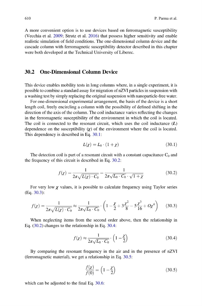
This dependency is described in Eq. 30.1:
L χ
ð Þ ¼ L 0 Á 1 þ χ
ð
Þ
ð30:1Þ
The detection coil is part of a resonant circuit with a constant capacitance C 0 and
the frequency of this circuit is described in Eq. 30.2:
f χ
ð Þ ¼
1
2π
ffiffiffiffiffiffiffiffiffiffiffiffiffiffiffiffiffi ffi
L χ
ð Þ Á C 0
p
¼
1
2π
ffiffiffiffiffiffiffiffiffiffiffiffiffi ffi
L 0 Á C 0
p
Á
ffiffiffiffiffiffiffiffiffiffiffi
1 þ χ
p
ð30:2Þ
For very low χ values, it is possible to calculate frequency using Taylor series
(Eq. 30.3):
f χ
ð Þ ¼
1
2π
ffiffiffiffiffiffiffiffiffiffiffiffiffiffiffiffiffi ffi
L χ
ð Þ Á C 0
p
%
1
2π
ffiffiffiffiffiffiffiffiffiffiffiffiffi ffi
L 0 Á C 0
p
Á 1 À
χ
2
þ 3
χ
2
8
À 5
χ
3
16
þ Oχ
4
ð30:3Þ
When neglecting items from the second order above, then the relationship in
Eq. (30.2) changes to the relationship in Eq. 30.4:
f χ
ð Þ %
1
2π
ffiffiffiffiffiffiffiffiffiffiffiffiffi ffi
L 0 Á C 0
p
Á 1 À
χ
2
ð30:4Þ
By comparing the resonant frequency in the air and in the presence of nZVI
(ferromagnetic material), we get a relationship in Eq. 30.5:
f χ
ð Þ
f 0
ð Þ
¼ 1 À
χ
2
ð30:5Þ
which can be adjusted to the final Eq. 30.6:
610
P. Parma et al.