

60
K. Deng et al.
c(i) =
⎡
⎣
cosθ i + u 2
x (1 − cosθ i )
u x u y (1 − cosθ i ) − u z sinθ i u x u z (1 − cosθ i ) + u y sinθ i
u y u x (1 − cosθ i ) + u z sinθ i cosθ i + u 2
y (1 − cosθ i ) u y u z (1 − cosθ i ) − u x sinθ i
u z u x (1 − cosθ i ) − u y sinθ i u z u y (1 − cosθ i ) + u x sinθ i cosθ i + u 2
z (1 − cosθ i )
⎤
⎦ ,
where u is the joint’s axis of rotation vector.
3 Results
3.1 Muscle Parameters
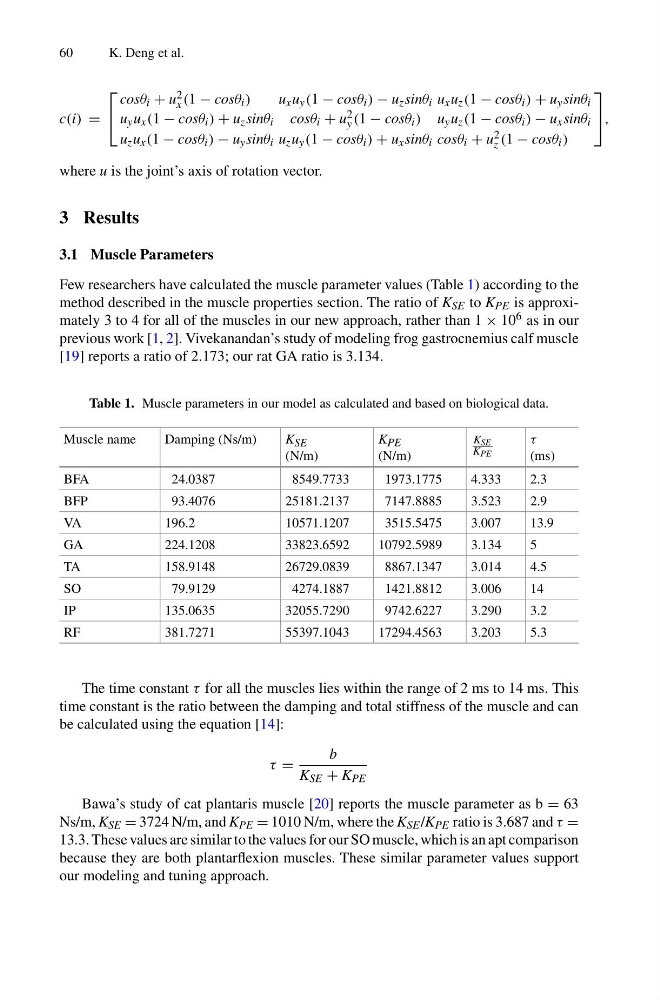
Few researchers have calculated the muscle parameter values (Table 1) according to the
method described in the muscle properties section. The ratio of K SE to K PE is approximately 3 to 4 for all of the muscles in our new approach, rather than 1 × 10 6 as in our
previous work [1, 2]. Vivekanandan’s study of modeling frog gastrocnemius calf muscle
[19] reports a ratio of 2.173; our rat GA ratio is 3.134.
Table 1. Muscle parameters in our model as calculated and based on biological data.
Muscle name
Damping (Ns/m)
K SE
(N/m)
K PE
(N/m)
K SE
K PE
τ
(ms)
BFA
24.0387
8549.7733
1973.1775
4.333
2.3
BFP
93.4076
25181.2137
7147.8885
3.523
2.9
VA
196.2
10571.1207
3515.5475
3.007
13.9
GA
224.1208
33823.6592
10792.5989
3.134
5
TA
158.9148
26729.0839
8867.1347
3.014
4.5
SO
79.9129
4274.1887
1421.8812
3.006
14
IP
135.0635
32055.7290
9742.6227
3.290
3.2
RF
381.7271
55397.1043
17294.4563
3.203
5.3
The time constant τ for all the muscles lies within the range of 2 ms to 14 ms. This
time constant is the ratio between the damping and total stiffness of the muscle and can
be calculated using the equation [14]:
τ =
b
K SE + K PE
Bawa’s study of cat plantaris muscle [20] reports the muscle parameter as b = 63
Ns/m, K SE = 3724 N/m, and K PE = 1010 N/m, where the K SE /K PE ratio is 3.687 and τ =
13.3. These values are similar to the values for our SO muscle, which is an apt comparison
because they are both plantarflexion muscles. These similar parameter values support
our modeling and tuning approach.
K. Deng et al.
c(i) =
⎡
⎣
cosθ i + u 2
x (1 − cosθ i )
u x u y (1 − cosθ i ) − u z sinθ i u x u z (1 − cosθ i ) + u y sinθ i
u y u x (1 − cosθ i ) + u z sinθ i cosθ i + u 2
y (1 − cosθ i ) u y u z (1 − cosθ i ) − u x sinθ i
u z u x (1 − cosθ i ) − u y sinθ i u z u y (1 − cosθ i ) + u x sinθ i cosθ i + u 2
z (1 − cosθ i )
⎤
⎦ ,
where u is the joint’s axis of rotation vector.
3 Results
3.1 Muscle Parameters
Few researchers have calculated the muscle parameter values (Table 1) according to the
method described in the muscle properties section. The ratio of K SE to K PE is approximately 3 to 4 for all of the muscles in our new approach, rather than 1 × 10 6 as in our
previous work [1, 2]. Vivekanandan’s study of modeling frog gastrocnemius calf muscle
[19] reports a ratio of 2.173; our rat GA ratio is 3.134.
Table 1. Muscle parameters in our model as calculated and based on biological data.
Muscle name
Damping (Ns/m)
K SE
(N/m)
K PE
(N/m)
K SE
K PE
τ
(ms)
BFA
24.0387
8549.7733
1973.1775
4.333
2.3
BFP
93.4076
25181.2137
7147.8885
3.523
2.9
VA
196.2
10571.1207
3515.5475
3.007
13.9
GA
224.1208
33823.6592
10792.5989
3.134
5
TA
158.9148
26729.0839
8867.1347
3.014
4.5
SO
79.9129
4274.1887
1421.8812
3.006
14
IP
135.0635
32055.7290
9742.6227
3.290
3.2
RF
381.7271
55397.1043
17294.4563
3.203
5.3
The time constant τ for all the muscles lies within the range of 2 ms to 14 ms. This
time constant is the ratio between the damping and total stiffness of the muscle and can
be calculated using the equation [14]:
τ =
b
K SE + K PE
Bawa’s study of cat plantaris muscle [20] reports the muscle parameter as b = 63
Ns/m, K SE = 3724 N/m, and K PE = 1010 N/m, where the K SE /K PE ratio is 3.687 and τ =
13.3. These values are similar to the values for our SO muscle, which is an apt comparison
because they are both plantarflexion muscles. These similar parameter values support
our modeling and tuning approach.