

58
K. Deng et al.
femoris (RF), which link the hip and knee joint; and Gastrocnemii (GA), which spans
the knee and ankle joint.
2.2 Length-Tension Curve
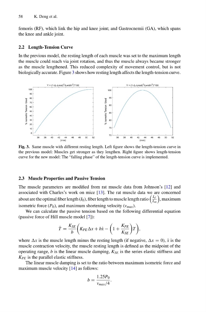
In the previous model, the resting length of each muscle was set to the maximum length
the muscle could reach via joint rotation, and thus the muscle always became stronger
as the muscle lengthened. This reduced complexity of movement control, but is not
biologically accurate. Figure 3 shows how resting length affects the length-tension curve.
Fig. 3. Same muscle with different resting length. Left figure shows the length-tension curve in
the previous model: Muscles get stronger as they lengthen. Right figure shows length-tension
curve for the new model: The “falling phase” of the length-tension curve is implemented.
2.3 Muscle Properties and Passive Tension
The muscle parameters are modified from rat muscle data from Johnson’s [12] and
associated with Charles’s work on mice [13]. The rat muscle data we are concerned
about are the optimal fiber length (I 0 ), fiber length to muscle length ratio
L f
L m
, maximum
isometric force (P 0 ), and maximum shortening velocity (v max ).
We can calculate the passive tension based on the following differential equation
(passive force of Hill muscle model [7]):
˙
T =
K SE
b
K PE x + b˙ x −
1 +
K PE
K SE
T
,
where x is the muscle length minus the resting length (if negative, x = 0), ˙
x is the
muscle contraction velocity, the muscle resting length is defined as the midpoint of the
operating range, b is the linear muscle damping, K SE is the series elastic stiffness and
K PE is the parallel elastic stiffness.
The linear muscle damping is set to the ratio between maximum isometric force and
maximum muscle velocity [14] as follows:
b =
1.25P 0
v max /4
.
K. Deng et al.
femoris (RF), which link the hip and knee joint; and Gastrocnemii (GA), which spans
the knee and ankle joint.
2.2 Length-Tension Curve
In the previous model, the resting length of each muscle was set to the maximum length
the muscle could reach via joint rotation, and thus the muscle always became stronger
as the muscle lengthened. This reduced complexity of movement control, but is not
biologically accurate. Figure 3 shows how resting length affects the length-tension curve.
Fig. 3. Same muscle with different resting length. Left figure shows the length-tension curve in
the previous model: Muscles get stronger as they lengthen. Right figure shows length-tension
curve for the new model: The “falling phase” of the length-tension curve is implemented.
2.3 Muscle Properties and Passive Tension
The muscle parameters are modified from rat muscle data from Johnson’s [12] and
associated with Charles’s work on mice [13]. The rat muscle data we are concerned
about are the optimal fiber length (I 0 ), fiber length to muscle length ratio
L f
L m
, maximum
isometric force (P 0 ), and maximum shortening velocity (v max ).
We can calculate the passive tension based on the following differential equation
(passive force of Hill muscle model [7]):
˙
T =
K SE
b
K PE x + b˙ x −
1 +
K PE
K SE
T
,
where x is the muscle length minus the resting length (if negative, x = 0), ˙
x is the
muscle contraction velocity, the muscle resting length is defined as the midpoint of the
operating range, b is the linear muscle damping, K SE is the series elastic stiffness and
K PE is the parallel elastic stiffness.
The linear muscle damping is set to the ratio between maximum isometric force and
maximum muscle velocity [14] as follows:
b =
1.25P 0
v max /4
.