

404
F. Young et al.
these limitations, a method is first described for defining muscle parameters that allow
us to then analyze the length-activation relationships for discontinuities. Understanding
the limitations formalized in this work is important when developing a neuromechanical
model in Animatlab.
2 Modeling Methods
2.1 The Linear Hill Muscle Model
Muscle models relate muscle length, velocity, stimulation, and tension with varying
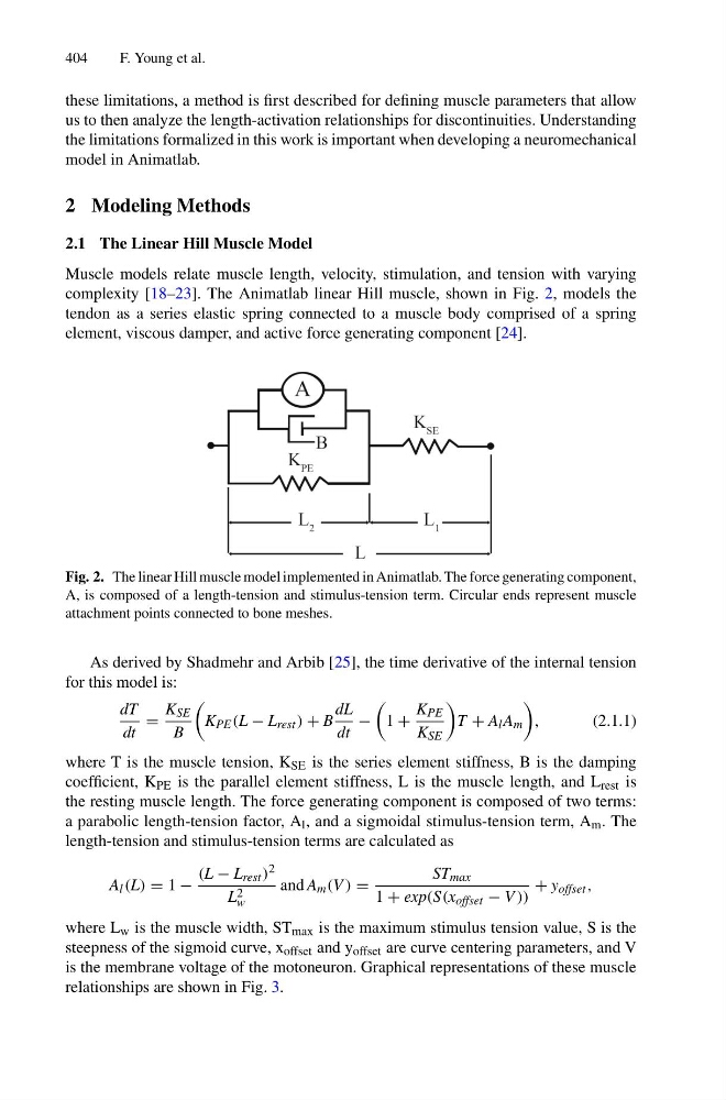
complexity [18–23]. The Animatlab linear Hill muscle, shown in Fig. 2, models the
tendon as a series elastic spring connected to a muscle body comprised of a spring
element, viscous damper, and active force generating component [24].
Fig. 2. The linear Hill muscle model implemented in Animatlab. The force generating component,
A, is composed of a length-tension and stimulus-tension term. Circular ends represent muscle
attachment points connected to bone meshes.
As derived by Shadmehr and Arbib [25], the time derivative of the internal tension
for this model is:
dT
dt
=
K SE
B
K PE (L − L rest ) + B
dL
dt
−
1 +
K PE
K SE
T + A l A m
,
(2.1.1)
where T is the muscle tension, K SE is the series element stiffness, B is the damping
coefficient, K PE is the parallel element stiffness, L is the muscle length, and L rest is
the resting muscle length. The force generating component is composed of two terms:
a parabolic length-tension factor, A l , and a sigmoidal stimulus-tension term, A m . The
length-tension and stimulus-tension terms are calculated as
A l (L) = 1 −
(L − L rest ) 2
L 2
w
and A m (V ) =
ST max
1 + exp(S(x offset − V ))
+ y offset ,
where L w is the muscle width, ST max is the maximum stimulus tension value, S is the
steepness of the sigmoid curve, x offset and y offset are curve centering parameters, and V
is the membrane voltage of the motoneuron. Graphical representations of these muscle
relationships are shown in Fig. 3.
F. Young et al.
these limitations, a method is first described for defining muscle parameters that allow
us to then analyze the length-activation relationships for discontinuities. Understanding
the limitations formalized in this work is important when developing a neuromechanical
model in Animatlab.
2 Modeling Methods
2.1 The Linear Hill Muscle Model
Muscle models relate muscle length, velocity, stimulation, and tension with varying
complexity [18–23]. The Animatlab linear Hill muscle, shown in Fig. 2, models the
tendon as a series elastic spring connected to a muscle body comprised of a spring
element, viscous damper, and active force generating component [24].
Fig. 2. The linear Hill muscle model implemented in Animatlab. The force generating component,
A, is composed of a length-tension and stimulus-tension term. Circular ends represent muscle
attachment points connected to bone meshes.
As derived by Shadmehr and Arbib [25], the time derivative of the internal tension
for this model is:
dT
dt
=
K SE
B
K PE (L − L rest ) + B
dL
dt
−
1 +
K PE
K SE
T + A l A m
,
(2.1.1)
where T is the muscle tension, K SE is the series element stiffness, B is the damping
coefficient, K PE is the parallel element stiffness, L is the muscle length, and L rest is
the resting muscle length. The force generating component is composed of two terms:
a parabolic length-tension factor, A l , and a sigmoidal stimulus-tension term, A m . The
length-tension and stimulus-tension terms are calculated as
A l (L) = 1 −
(L − L rest ) 2
L 2
w
and A m (V ) =
ST max
1 + exp(S(x offset − V ))
+ y offset ,
where L w is the muscle width, ST max is the maximum stimulus tension value, S is the
steepness of the sigmoid curve, x offset and y offset are curve centering parameters, and V
is the membrane voltage of the motoneuron. Graphical representations of these muscle
relationships are shown in Fig. 3.