

346
N. S. Szczecinski et al.
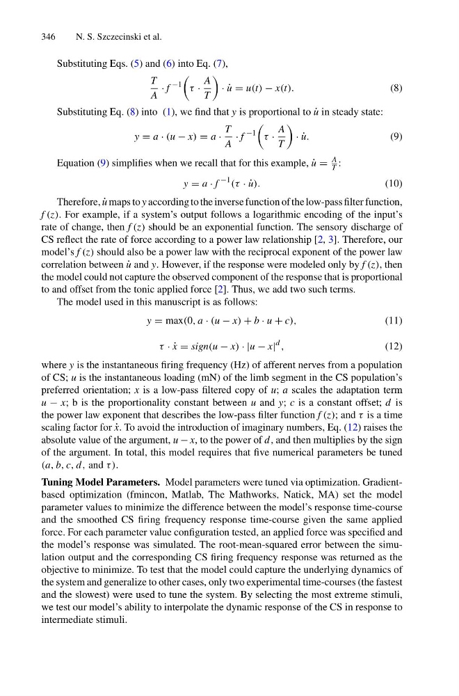
Substituting Eqs. (5) and (6) into Eq. (7),
T
A
· f
−1
τ ·
A
T
· ˙
u = u(t) − x(t).
(8)
Substituting Eq. (8) into (1), we find that y is proportional to ˙
u in steady state:
y = a · (u − x) = a ·
T
A
· f
−1
τ ·
A
T
· ˙
u.
(9)
Equation (9) simplifies when we recall that for this example, ˙
u =
A
T :
y = a · f
−1
(τ · ˙
u).
(10)
Therefore, ˙
u maps to y according to the inverse function of the low-pass filter function,
f (z). For example, if a system’s output follows a logarithmic encoding of the input’s
rate of change, then f (z) should be an exponential function. The sensory discharge of
CS reflect the rate of force according to a power law relationship [2, 3]. Therefore, our
model’s f (z) should also be a power law with the reciprocal exponent of the power law
correlation between ˙
u and y. However, if the response were modeled only by f (z), then
the model could not capture the observed component of the response that is proportional
to and offset from the tonic applied force [2]. Thus, we add two such terms.
The model used in this manuscript is as follows:
y = max(0, a · (u − x) + b · u + c),
(11)
τ · ˙
x = sign(u − x) · |u − x|
d
,
(12)
where y is the instantaneous firing frequency (Hz) of afferent nerves from a population
of CS; u is the instantaneous loading (mN) of the limb segment in the CS population’s
preferred orientation; x is a low-pass filtered copy of u; a scales the adaptation term
u − x; b is the proportionality constant between u and y; c is a constant offset; d is
the power law exponent that describes the low-pass filter function f (z); and τ is a time
scaling factor for ˙
x. To avoid the introduction of imaginary numbers, Eq. (12) raises the
absolute value of the argument, u − x, to the power of d , and then multiplies by the sign
of the argument. In total, this model requires that five numerical parameters be tuned
(a, b, c, d , and τ ).
Tuning Model Parameters. Model parameters were tuned via optimization. Gradientbased optimization (fmincon, Matlab, The Mathworks, Natick, MA) set the model
parameter values to minimize the difference between the model’s response time-course
and the smoothed CS firing frequency response time-course given the same applied
force. For each parameter value configuration tested, an applied force was specified and
the model’s response was simulated. The root-mean-squared error between the simulation output and the corresponding CS firing frequency response was returned as the
objective to minimize. To test that the model could capture the underlying dynamics of
the system and generalize to other cases, only two experimental time-courses (the fastest
and the slowest) were used to tune the system. By selecting the most extreme stimuli,
we test our model’s ability to interpolate the dynamic response of the CS in response to
intermediate stimuli.
N. S. Szczecinski et al.
Substituting Eqs. (5) and (6) into Eq. (7),
T
A
· f
−1
τ ·
A
T
· ˙
u = u(t) − x(t).
(8)
Substituting Eq. (8) into (1), we find that y is proportional to ˙
u in steady state:
y = a · (u − x) = a ·
T
A
· f
−1
τ ·
A
T
· ˙
u.
(9)
Equation (9) simplifies when we recall that for this example, ˙
u =
A
T :
y = a · f
−1
(τ · ˙
u).
(10)
Therefore, ˙
u maps to y according to the inverse function of the low-pass filter function,
f (z). For example, if a system’s output follows a logarithmic encoding of the input’s
rate of change, then f (z) should be an exponential function. The sensory discharge of
CS reflect the rate of force according to a power law relationship [2, 3]. Therefore, our
model’s f (z) should also be a power law with the reciprocal exponent of the power law
correlation between ˙
u and y. However, if the response were modeled only by f (z), then
the model could not capture the observed component of the response that is proportional
to and offset from the tonic applied force [2]. Thus, we add two such terms.
The model used in this manuscript is as follows:
y = max(0, a · (u − x) + b · u + c),
(11)
τ · ˙
x = sign(u − x) · |u − x|
d
,
(12)
where y is the instantaneous firing frequency (Hz) of afferent nerves from a population
of CS; u is the instantaneous loading (mN) of the limb segment in the CS population’s
preferred orientation; x is a low-pass filtered copy of u; a scales the adaptation term
u − x; b is the proportionality constant between u and y; c is a constant offset; d is
the power law exponent that describes the low-pass filter function f (z); and τ is a time
scaling factor for ˙
x. To avoid the introduction of imaginary numbers, Eq. (12) raises the
absolute value of the argument, u − x, to the power of d , and then multiplies by the sign
of the argument. In total, this model requires that five numerical parameters be tuned
(a, b, c, d , and τ ).
Tuning Model Parameters. Model parameters were tuned via optimization. Gradientbased optimization (fmincon, Matlab, The Mathworks, Natick, MA) set the model
parameter values to minimize the difference between the model’s response time-course
and the smoothed CS firing frequency response time-course given the same applied
force. For each parameter value configuration tested, an applied force was specified and
the model’s response was simulated. The root-mean-squared error between the simulation output and the corresponding CS firing frequency response was returned as the
objective to minimize. To test that the model could capture the underlying dynamics of
the system and generalize to other cases, only two experimental time-courses (the fastest
and the slowest) were used to tune the system. By selecting the most extreme stimuli,
we test our model’s ability to interpolate the dynamic response of the CS in response to
intermediate stimuli.