

Modeling the Dynamic Sensory Discharges of Insect CS
345
the long-term history of the input be calculated? In the following, we demonstrate how
the properties of a low-pass filter inform the correlation between the total response and
the rate of change of the input. Then, we show that a power law low-pass filter matches
the response of CS.
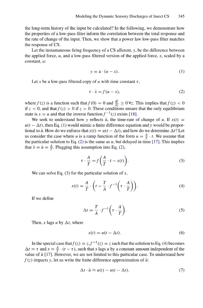
Let the instantaneous firing frequency of a CS afferent, y, be the difference between
the applied force, u, and a low-pass filtered version of the applied force, x, scaled by a
constant, a:
y = a · (u − x).
(1)
Let x be a low-pass filtered copy of u with time constant τ ,
τ · ˙
x = f (u − x),
(2)
where f (z) is a function such that f (0) = 0 and
df
dz ≥ 0 ∀z. This implies that f (z) < 0
if z < 0, and that f (z) > 0 if z > 0. These conditions ensure that the only equilibrium
state is x = u and that the inverse function f −1 (z) exists [18].
We seek to understand how y reflects ˙
u, the time-rate of change of u. If x(t) =
u(t − t), then Eq. (1) would mimic a finite difference equation and y would be proportional to ˙
u. How do we enforce that x(t) = u(t − t), and how do we determine t? Let
us consider the case where u is a ramp function of the form u =
A
T · t. We assume that
the particular solution to Eq. (2) is the same as u, but delayed in time [17]. This implies
that ˙
x = ˙
u =
A
T . Plugging this assumption into Eq. (2),
τ ·
A
T
= f
A
T
· t − x(t)
.
(3)
We can solve Eq. (3) for the particular solution of x,
x(t) =
A
T
·
t −
T
A
· f
−1
τ ·
A
T
.
(4)
If we define
t =
T
A
· f
−1
τ ·
A
T
.
(5)
Then, x lags u by t, where
x(t) = u(t − t).
(6)
In the special case that f (z) = z, f −1 (z) = z such that the solution to Eq. (4) becomes
t = τ and x =
A
T · (t − τ ), such that x lags u by a constant amount independent of the
value of ˙
u [17]. However, we are not limited to this particular case. To understand how
f (z) impacts y, let us write the finite difference approximation of ˙
u:
t · ˙
u ≈ u(t) − u(t − t).
(7)
345
the long-term history of the input be calculated? In the following, we demonstrate how
the properties of a low-pass filter inform the correlation between the total response and
the rate of change of the input. Then, we show that a power law low-pass filter matches
the response of CS.
Let the instantaneous firing frequency of a CS afferent, y, be the difference between
the applied force, u, and a low-pass filtered version of the applied force, x, scaled by a
constant, a:
y = a · (u − x).
(1)
Let x be a low-pass filtered copy of u with time constant τ ,
τ · ˙
x = f (u − x),
(2)
where f (z) is a function such that f (0) = 0 and
df
dz ≥ 0 ∀z. This implies that f (z) < 0
if z < 0, and that f (z) > 0 if z > 0. These conditions ensure that the only equilibrium
state is x = u and that the inverse function f −1 (z) exists [18].
We seek to understand how y reflects ˙
u, the time-rate of change of u. If x(t) =
u(t − t), then Eq. (1) would mimic a finite difference equation and y would be proportional to ˙
u. How do we enforce that x(t) = u(t − t), and how do we determine t? Let
us consider the case where u is a ramp function of the form u =
A
T · t. We assume that
the particular solution to Eq. (2) is the same as u, but delayed in time [17]. This implies
that ˙
x = ˙
u =
A
T . Plugging this assumption into Eq. (2),
τ ·
A
T
= f
A
T
· t − x(t)
.
(3)
We can solve Eq. (3) for the particular solution of x,
x(t) =
A
T
·
t −
T
A
· f
−1
τ ·
A
T
.
(4)
If we define
t =
T
A
· f
−1
τ ·
A
T
.
(5)
Then, x lags u by t, where
x(t) = u(t − t).
(6)
In the special case that f (z) = z, f −1 (z) = z such that the solution to Eq. (4) becomes
t = τ and x =
A
T · (t − τ ), such that x lags u by a constant amount independent of the
value of ˙
u [17]. However, we are not limited to this particular case. To understand how
f (z) impacts y, let us write the finite difference approximation of ˙
u:
t · ˙
u ≈ u(t) − u(t − t).
(7)