

332
J. Stankiewicz and B. Webb
3 Results
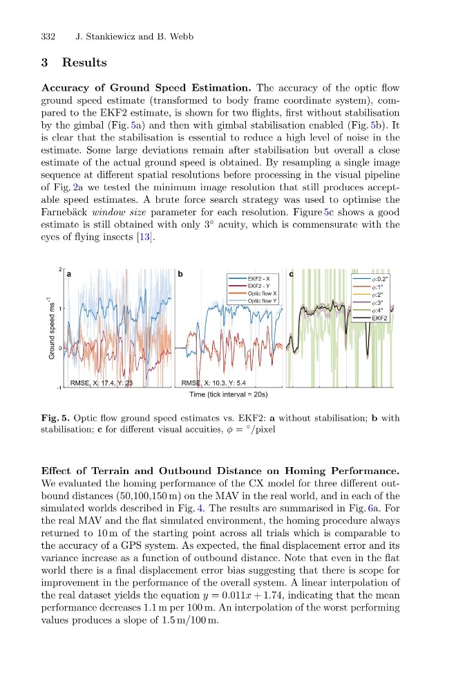
Accuracy of Ground Speed Estimation. The accuracy of the optic flow
ground speed estimate (transformed to body frame coordinate system), compared to the EKF2 estimate, is shown for two flights, first without stabilisation
by the gimbal (Fig. 5a) and then with gimbal stabilisation enabled (Fig. 5b). It
is clear that the stabilisation is essential to reduce a high level of noise in the
estimate. Some large deviations remain after stabilisation but overall a close
estimate of the actual ground speed is obtained. By resampling a single image
sequence at different spatial resolutions before processing in the visual pipeline
of Fig. 2a we tested the minimum image resolution that still produces acceptable speed estimates. A brute force search strategy was used to optimise the
Farneb¨ ack window size parameter for each resolution. Figure 5c shows a good
estimate is still obtained with only 3
◦ acuity, which is commensurate with the
eyes of flying insects [13].
-1
0
1
2
Ground speed ms
-1
RMSE, X: 17.4, Y: 23
Time (tick interval = 20s)
RMSE, X: 10.3, Y: 5.4
EKF2 - X
EKF2 - Y
Optic flow X
Optic flow Y
:0.2°
:1°
:2°
:3°
:4°
EKF2
a
b
c
Fig. 5. Optic flow ground speed estimates vs. EKF2: a without stabilisation; b with
stabilisation; c for different visual accuities, φ =
◦ /pixel
Effect of Terrain and Outbound Distance on Homing Performance.
We evaluated the homing performance of the CX model for three different outbound distances (50,100,150 m) on the MAV in the real world, and in each of the
simulated worlds described in Fig. 4. The results are summarised in Fig. 6a. For
the real MAV and the flat simulated environment, the homing procedure always
returned to 10 m of the starting point across all trials which is comparable to
the accuracy of a GPS system. As expected, the final displacement error and its
variance increase as a function of outbound distance. Note that even in the flat
world there is a final displacement error bias suggesting that there is scope for
improvement in the performance of the overall system. A linear interpolation of
the real dataset yields the equation y = 0.011x + 1.74, indicating that the mean
performance decreases 1.1 m per 100 m. An interpolation of the worst performing
values produces a slope of 1.5 m/100 m.
J. Stankiewicz and B. Webb
3 Results
Accuracy of Ground Speed Estimation. The accuracy of the optic flow
ground speed estimate (transformed to body frame coordinate system), compared to the EKF2 estimate, is shown for two flights, first without stabilisation
by the gimbal (Fig. 5a) and then with gimbal stabilisation enabled (Fig. 5b). It
is clear that the stabilisation is essential to reduce a high level of noise in the
estimate. Some large deviations remain after stabilisation but overall a close
estimate of the actual ground speed is obtained. By resampling a single image
sequence at different spatial resolutions before processing in the visual pipeline
of Fig. 2a we tested the minimum image resolution that still produces acceptable speed estimates. A brute force search strategy was used to optimise the
Farneb¨ ack window size parameter for each resolution. Figure 5c shows a good
estimate is still obtained with only 3
◦ acuity, which is commensurate with the
eyes of flying insects [13].
-1
0
1
2
Ground speed ms
-1
RMSE, X: 17.4, Y: 23
Time (tick interval = 20s)
RMSE, X: 10.3, Y: 5.4
EKF2 - X
EKF2 - Y
Optic flow X
Optic flow Y
:0.2°
:1°
:2°
:3°
:4°
EKF2
a
b
c
Fig. 5. Optic flow ground speed estimates vs. EKF2: a without stabilisation; b with
stabilisation; c for different visual accuities, φ =
◦ /pixel
Effect of Terrain and Outbound Distance on Homing Performance.
We evaluated the homing performance of the CX model for three different outbound distances (50,100,150 m) on the MAV in the real world, and in each of the
simulated worlds described in Fig. 4. The results are summarised in Fig. 6a. For
the real MAV and the flat simulated environment, the homing procedure always
returned to 10 m of the starting point across all trials which is comparable to
the accuracy of a GPS system. As expected, the final displacement error and its
variance increase as a function of outbound distance. Note that even in the flat
world there is a final displacement error bias suggesting that there is scope for
improvement in the performance of the overall system. A linear interpolation of
the real dataset yields the equation y = 0.011x + 1.74, indicating that the mean
performance decreases 1.1 m per 100 m. An interpolation of the worst performing
values produces a slope of 1.5 m/100 m.