

224
K. Kodono and H. Kimura
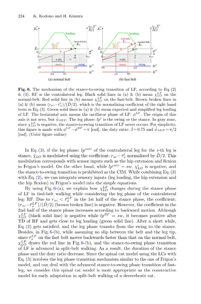
Fig. 6. The mechanism of the stance-to-swing transition of LF, according to Eq. (2)
& (3). RF is the contralateral leg. Black solid lines in (a) & (b) mean χ
LF
LO on the
normal-belt. Red solid line in (b) means χ
LF
LO on the fast-belt. Brown broken lines in
(a) & (b) mean (rxc−¯ r
i
x )/( ˆ
D/2), which is the normalizing coefficient of the right hand
term in Eq. (3). Green solid lines in (a) & (b) mean expected and simplified leg loading
of LF. The horizontal axis means the oscillator phase of LF: φ
LF . The origin of this
axis is not zero, but ˆ
φAEP . The leg phase: lp
i is the swing or the stance. In gray zone,
since χ
LF
LO is negative, the stance-to-swing transition of LF never occurs. For simplicity,
this figure is made with φ
LF −φ
RF = π [rad], the duty ratio: ˆ
β = 0.75 and ˆ
φAEP = π/2
[rad]. (Color figure online)
In Eq. (3), if the leg phase: lp
cntr of the contralateral leg for the i-th leg is
stance, ˆ
χ LO is modulated using the coefficient: r xc − ¯
r
i
x normalized by ˆ
D/2. This
modulation corresponds with sensor inputs such as the hip extension and flexion
in Frigon’s model. On the other hand, while lp
cntr = sw, χ
i
LO is negative, and
the stance-to-swing transition is prohibited as the CIM. While combining Eq. (3)
with Eq. (2), we can integrate sensory inputs (leg loading, the hip extension and
the hip flexion) in Frigon’s model into the simple equations.
By using Fig. 6-(a), we explain how χ
LF
LO changes during the stance phase
of LF in tied-belt walking while considering the leg phase of the contralateral
leg: RF. Due to r xc < ¯
r
LF
x
in the 1st half of the stance phase, the coefficient:
(r xc −¯ r
LF
x )/( ˆ
D/2) (brown broken line) is negative. However, the coefficient in the
2nd half of the stance phase increases according to backward motion. Although
χ
LF
LO (black solid line) is negative while lp
RF = sw, it becomes positive after
TD of RF and gets close to leg loading (green solid line). After a short while,
Eq. (2) gets satisfied, and the leg phase transits from the swing to the stance.
Besides, in Fig. 6-(b), while assuming no slip between the belt and the leg tip,
since ¯
r
LF
x
on the fast belt moves backwards faster than that on the normal belt,
χ
LF
LO draws the red line in Fig. 6-(b), and the stance-to-swing phase transition
of LF is advanced in split-belt walking. As a result, the duration of the stance
phase and the duty ratio decrease. Since the spinal cat model using the LCs with
Eq. (3) involves the leg phase transition mechanism similar to the one of Frigon’s
model, and can deal with the advanced stance-to-swing phase transition of fastleg, we consider this spinal cat model is most appropriate as the constructive
model for early adaptation in split-belt walking of a decerebrate cat.
K. Kodono and H. Kimura
Fig. 6. The mechanism of the stance-to-swing transition of LF, according to Eq. (2)
& (3). RF is the contralateral leg. Black solid lines in (a) & (b) mean χ
LF
LO on the
normal-belt. Red solid line in (b) means χ
LF
LO on the fast-belt. Brown broken lines in
(a) & (b) mean (rxc−¯ r
i
x )/( ˆ
D/2), which is the normalizing coefficient of the right hand
term in Eq. (3). Green solid lines in (a) & (b) mean expected and simplified leg loading
of LF. The horizontal axis means the oscillator phase of LF: φ
LF . The origin of this
axis is not zero, but ˆ
φAEP . The leg phase: lp
i is the swing or the stance. In gray zone,
since χ
LF
LO is negative, the stance-to-swing transition of LF never occurs. For simplicity,
this figure is made with φ
LF −φ
RF = π [rad], the duty ratio: ˆ
β = 0.75 and ˆ
φAEP = π/2
[rad]. (Color figure online)
In Eq. (3), if the leg phase: lp
cntr of the contralateral leg for the i-th leg is
stance, ˆ
χ LO is modulated using the coefficient: r xc − ¯
r
i
x normalized by ˆ
D/2. This
modulation corresponds with sensor inputs such as the hip extension and flexion
in Frigon’s model. On the other hand, while lp
cntr = sw, χ
i
LO is negative, and
the stance-to-swing transition is prohibited as the CIM. While combining Eq. (3)
with Eq. (2), we can integrate sensory inputs (leg loading, the hip extension and
the hip flexion) in Frigon’s model into the simple equations.
By using Fig. 6-(a), we explain how χ
LF
LO changes during the stance phase
of LF in tied-belt walking while considering the leg phase of the contralateral
leg: RF. Due to r xc < ¯
r
LF
x
in the 1st half of the stance phase, the coefficient:
(r xc −¯ r
LF
x )/( ˆ
D/2) (brown broken line) is negative. However, the coefficient in the
2nd half of the stance phase increases according to backward motion. Although
χ
LF
LO (black solid line) is negative while lp
RF = sw, it becomes positive after
TD of RF and gets close to leg loading (green solid line). After a short while,
Eq. (2) gets satisfied, and the leg phase transits from the swing to the stance.
Besides, in Fig. 6-(b), while assuming no slip between the belt and the leg tip,
since ¯
r
LF
x
on the fast belt moves backwards faster than that on the normal belt,
χ
LF
LO draws the red line in Fig. 6-(b), and the stance-to-swing phase transition
of LF is advanced in split-belt walking. As a result, the duration of the stance
phase and the duty ratio decrease. Since the spinal cat model using the LCs with
Eq. (3) involves the leg phase transition mechanism similar to the one of Frigon’s
model, and can deal with the advanced stance-to-swing phase transition of fastleg, we consider this spinal cat model is most appropriate as the constructive
model for early adaptation in split-belt walking of a decerebrate cat.