

A Framework for Resolving Motivational Conflict via Attractor Dynamics
197
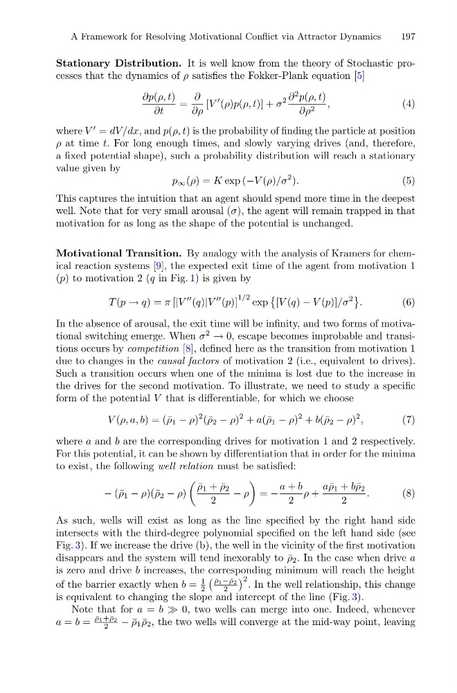
Stationary Distribution. It is well know from the theory of Stochastic processes that the dynamics of ρ satisfies the Fokker-Plank equation [5]
∂p(ρ, t)
∂t
=
∂
∂ρ
[V
(ρ)p(ρ, t)] + σ
2 ∂
2 p(ρ, t)
∂ρ 2 ,
(4)
where V
= dV /dx, and p(ρ, t) is the probability of finding the particle at position
ρ at time t. For long enough times, and slowly varying drives (and, therefore,
a fixed potential shape), such a probability distribution will reach a stationary
value given by
p ∞ (ρ) = K exp (−V (ρ)/σ
2 ).
(5)
This captures the intuition that an agent should spend more time in the deepest
well. Note that for very small arousal (σ), the agent will remain trapped in that
motivation for as long as the shape of the potential is unchanged.
Motivational Transition. By analogy with the analysis of Kramers for chemical reaction systems [9], the expected exit time of the agent from motivation 1
(p) to motivation 2 (q in Fig. 1) is given by
T (p → q) = π [|V
(q)|V
(p)]
1/2 exp
[V (q) − V (p)]/σ
2
.
(6)
In the absence of arousal, the exit time will be infinity, and two forms of motivational switching emerge. When σ
2
→ 0, escape becomes improbable and transitions occurs by competition [8], defined here as the transition from motivation 1
due to changes in the causal factors of motivation 2 (i.e., equivalent to drives).
Such a transition occurs when one of the minima is lost due to the increase in
the drives for the second motivation. To illustrate, we need to study a specific
form of the potential V that is differentiable, for which we choose
V (ρ, a, b) = (¯ ρ 1 − ρ)
2 (¯ ρ 2 − ρ)
2 + a(¯ ρ 1 − ρ)
2 + b(¯ ρ 2 − ρ)
2 ,
(7)
where a and b are the corresponding drives for motivation 1 and 2 respectively.
For this potential, it can be shown by differentiation that in order for the minima
to exist, the following well relation must be satisfied:
− (¯ ρ 1 − ρ)(¯ ρ 2 − ρ)
¯
ρ 1 + ¯
ρ 2
2
− ρ
= −
a + b
2
ρ +
a¯ ρ 1 + b¯ ρ 2
2
.
(8)
As such, wells will exist as long as the line specified by the right hand side
intersects with the third-degree polynomial specified on the left hand side (see
Fig. 3). If we increase the drive (b), the well in the vicinity of the first motivation
disappears and the system will tend inexorably to ¯
ρ 2 . In the case when drive a
is zero and drive b increases, the corresponding minimum will reach the height
of the barrier exactly when b =
1
2
¯
ρ1− ¯
ρ2
2
2 . In the well relationship, this change
is equivalent to changing the slope and intercept of the line (Fig. 3).
Note that for a = b 0, two wells can merge into one. Indeed, whenever
a = b =
¯
ρ1+¯ ρ2
2
− ¯
ρ 1 ¯
ρ 2 , the two wells will converge at the mid-way point, leaving
197
Stationary Distribution. It is well know from the theory of Stochastic processes that the dynamics of ρ satisfies the Fokker-Plank equation [5]
∂p(ρ, t)
∂t
=
∂
∂ρ
[V
(ρ)p(ρ, t)] + σ
2 ∂
2 p(ρ, t)
∂ρ 2 ,
(4)
where V
= dV /dx, and p(ρ, t) is the probability of finding the particle at position
ρ at time t. For long enough times, and slowly varying drives (and, therefore,
a fixed potential shape), such a probability distribution will reach a stationary
value given by
p ∞ (ρ) = K exp (−V (ρ)/σ
2 ).
(5)
This captures the intuition that an agent should spend more time in the deepest
well. Note that for very small arousal (σ), the agent will remain trapped in that
motivation for as long as the shape of the potential is unchanged.
Motivational Transition. By analogy with the analysis of Kramers for chemical reaction systems [9], the expected exit time of the agent from motivation 1
(p) to motivation 2 (q in Fig. 1) is given by
T (p → q) = π [|V
(q)|V
(p)]
1/2 exp
[V (q) − V (p)]/σ
2
.
(6)
In the absence of arousal, the exit time will be infinity, and two forms of motivational switching emerge. When σ
2
→ 0, escape becomes improbable and transitions occurs by competition [8], defined here as the transition from motivation 1
due to changes in the causal factors of motivation 2 (i.e., equivalent to drives).
Such a transition occurs when one of the minima is lost due to the increase in
the drives for the second motivation. To illustrate, we need to study a specific
form of the potential V that is differentiable, for which we choose
V (ρ, a, b) = (¯ ρ 1 − ρ)
2 (¯ ρ 2 − ρ)
2 + a(¯ ρ 1 − ρ)
2 + b(¯ ρ 2 − ρ)
2 ,
(7)
where a and b are the corresponding drives for motivation 1 and 2 respectively.
For this potential, it can be shown by differentiation that in order for the minima
to exist, the following well relation must be satisfied:
− (¯ ρ 1 − ρ)(¯ ρ 2 − ρ)
¯
ρ 1 + ¯
ρ 2
2
− ρ
= −
a + b
2
ρ +
a¯ ρ 1 + b¯ ρ 2
2
.
(8)
As such, wells will exist as long as the line specified by the right hand side
intersects with the third-degree polynomial specified on the left hand side (see
Fig. 3). If we increase the drive (b), the well in the vicinity of the first motivation
disappears and the system will tend inexorably to ¯
ρ 2 . In the case when drive a
is zero and drive b increases, the corresponding minimum will reach the height
of the barrier exactly when b =
1
2
¯
ρ1− ¯
ρ2
2
2 . In the well relationship, this change
is equivalent to changing the slope and intercept of the line (Fig. 3).
Note that for a = b 0, two wells can merge into one. Indeed, whenever
a = b =
¯
ρ1+¯ ρ2
2
− ¯
ρ 1 ¯
ρ 2 , the two wells will converge at the mid-way point, leaving