

86
J. Fan et al.
we use dynamic programming
1 with an up-sweep approach. This allows to transfer the optimization of the whole shape into a series of optimal sub-problems.
The problem is formalized as finding the minimum path (minimum number of
segments) from a certain point, p i , up to an ending point, p j (with i < j), both
selected from the set of sorted list of skeleton points P srt = {p 1 , p 2 , · · · , p M },
having the minimum fitting error defined as:
J (p i , p j ) = min
i
(5)
where J (p i , p j ) denotes the M × M cost matrix of fitting errors over the connected piece-wise segments. On the right hand of the equation, J (p i , p k ) denotes
the specific configuration from p i to a point p k which lies in between the start
and the end point. Similarly, J (p k , p j ) denotes the configuration from p k to the
endpoint p j .
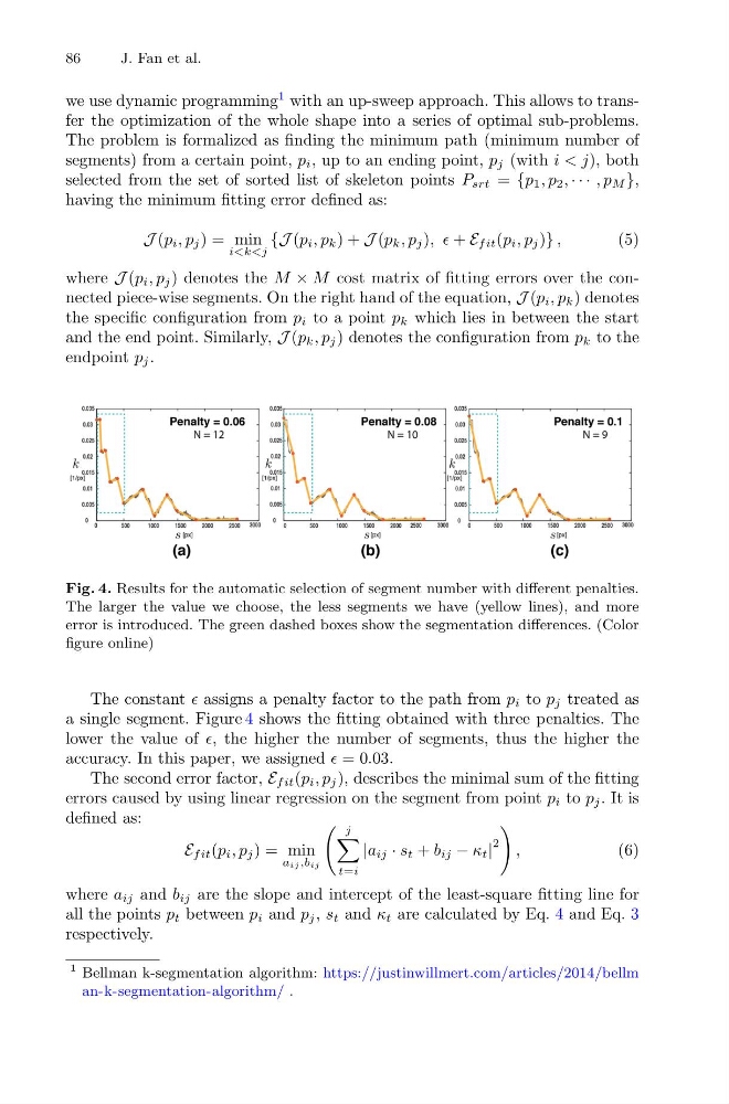
Fig. 4. Results for the automatic selection of segment number with different penalties.
The larger the value we choose, the less segments we have (yellow lines), and more
error is introduced. The green dashed boxes show the segmentation differences. (Color
figure online)
The constant assigns a penalty factor to the path from p i to p j treated as
a single segment. Figure 4 shows the fitting obtained with three penalties. The
lower the value of , the higher the number of segments, thus the higher the
accuracy. In this paper, we assigned = 0.03.
The second error factor, E fit (p i , p j ), describes the minimal sum of the fitting
errors caused by using linear regression on the segment from point p i to p j . It is
defined as:
E fit (p i , p j ) = min
aij ,bij
j
t=i
|a ij · s t + b ij − κ t |
2
,
(6)
where a ij and b ij are the slope and intercept of the least-square fitting line for
all the points p t between p i and p j , s t and κ t are calculated by Eq. 4 and Eq. 3
respectively.
1 Bellman k-segmentation algorithm: https://justinwillmert.com/articles/2014/bellm
an-k-segmentation-algorithm/ .
J. Fan et al.
we use dynamic programming
1 with an up-sweep approach. This allows to transfer the optimization of the whole shape into a series of optimal sub-problems.
The problem is formalized as finding the minimum path (minimum number of
segments) from a certain point, p i , up to an ending point, p j (with i < j), both
selected from the set of sorted list of skeleton points P srt = {p 1 , p 2 , · · · , p M },
having the minimum fitting error defined as:
J (p i , p j ) = min
i
(5)
where J (p i , p j ) denotes the M × M cost matrix of fitting errors over the connected piece-wise segments. On the right hand of the equation, J (p i , p k ) denotes
the specific configuration from p i to a point p k which lies in between the start
and the end point. Similarly, J (p k , p j ) denotes the configuration from p k to the
endpoint p j .
Fig. 4. Results for the automatic selection of segment number with different penalties.
The larger the value we choose, the less segments we have (yellow lines), and more
error is introduced. The green dashed boxes show the segmentation differences. (Color
figure online)
The constant assigns a penalty factor to the path from p i to p j treated as
a single segment. Figure 4 shows the fitting obtained with three penalties. The
lower the value of , the higher the number of segments, thus the higher the
accuracy. In this paper, we assigned = 0.03.
The second error factor, E fit (p i , p j ), describes the minimal sum of the fitting
errors caused by using linear regression on the segment from point p i to p j . It is
defined as:
E fit (p i , p j ) = min
aij ,bij
j
t=i
|a ij · s t + b ij − κ t |
2
,
(6)
where a ij and b ij are the slope and intercept of the least-square fitting line for
all the points p t between p i and p j , s t and κ t are calculated by Eq. 4 and Eq. 3
respectively.
1 Bellman k-segmentation algorithm: https://justinwillmert.com/articles/2014/bellm
an-k-segmentation-algorithm/ .