

16 Theoretical Foundations of Super-Resolution in Microspherical Nanoscopy
415
1
2
3
4
5
6
0
0.04
0.08
0.12
0.16
0.2
(|x
v |-R)/R
d/R
n s =1.4
1.6
1.7
2
3
4
5
6
7
0
0.04
0.08
0.12
0.16
0.2
(a)
( b )
M
d/R
n s =1.4
1.6
1.7
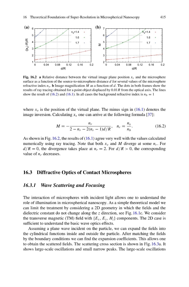
Fig. 16.2 a Relative distance between the virtual image plane position x v and the microsphere
surface as a function of the source-to-microsphere distance d for several values of the microsphere
refractive index n s . b Image magnification M as a function of d. The dots in both frames show the
results of ray tracing obtained for a point object displaced by 0.01R from the optical axis. The lines
show the result of (16.2) and (16.1). In all cases the background refractive index is n b = 1
where x v is the position of the virtual plane. The minus sign in (16.1) denotes the
image inversion. Calculating x v one can arrive at the following formula [37]:
M = −
n r
2 − n r − 2(n r − 1)d/R
, n r =
n s
n b
.
(16.2)
As shown in Fig. 16.2, the results of (16.1) agree very well with the values calculated
numerically using ray tracing. Note that both x v and M diverge at some n r . For
d/R = 0, the divergence takes place at n r = 2. For d/R > 0, the corresponding
value of n r decreases.
16.3 Diffractive Optics of Contact Microspheres
16.3.1 Wave Scattering and Focusing
The interaction of microspheres with incident light allows one to understand the
role of illumination in microspherical nanoscopy. As a simple theoretical model we
can limit the treatment by considering a 2D geometry in which the fields and the
dielectric constant do not change along the z direction, see Fig. 16.1c. We consider
the transverse magnetic (TM) field with {E x , E y , H z } components. The 2D case is
sufficient to understand the basic wave optics effects.
Assuming a plane wave incident on the particle, we can expand the fields into
the cylindrical functions inside and outside the particle. After matching the fields
by the boundary conditions we can find the expansion coefficients. This allows one
to obtain the scattered fields. The scattering cross section is shown in Fig. 16.3a. It
shows large-scale oscillations and small narrow peaks. The large-scale oscillations
415
1
2
3
4
5
6
0
0.04
0.08
0.12
0.16
0.2
(|x
v |-R)/R
d/R
n s =1.4
1.6
1.7
2
3
4
5
6
7
0
0.04
0.08
0.12
0.16
0.2
(a)
( b )
M
d/R
n s =1.4
1.6
1.7
Fig. 16.2 a Relative distance between the virtual image plane position x v and the microsphere
surface as a function of the source-to-microsphere distance d for several values of the microsphere
refractive index n s . b Image magnification M as a function of d. The dots in both frames show the
results of ray tracing obtained for a point object displaced by 0.01R from the optical axis. The lines
show the result of (16.2) and (16.1). In all cases the background refractive index is n b = 1
where x v is the position of the virtual plane. The minus sign in (16.1) denotes the
image inversion. Calculating x v one can arrive at the following formula [37]:
M = −
n r
2 − n r − 2(n r − 1)d/R
, n r =
n s
n b
.
(16.2)
As shown in Fig. 16.2, the results of (16.1) agree very well with the values calculated
numerically using ray tracing. Note that both x v and M diverge at some n r . For
d/R = 0, the divergence takes place at n r = 2. For d/R > 0, the corresponding
value of n r decreases.
16.3 Diffractive Optics of Contact Microspheres
16.3.1 Wave Scattering and Focusing
The interaction of microspheres with incident light allows one to understand the
role of illumination in microspherical nanoscopy. As a simple theoretical model we
can limit the treatment by considering a 2D geometry in which the fields and the
dielectric constant do not change along the z direction, see Fig. 16.1c. We consider
the transverse magnetic (TM) field with {E x , E y , H z } components. The 2D case is
sufficient to understand the basic wave optics effects.
Assuming a plane wave incident on the particle, we can expand the fields into
the cylindrical functions inside and outside the particle. After matching the fields
by the boundary conditions we can find the expansion coefficients. This allows one
to obtain the scattered fields. The scattering cross section is shown in Fig. 16.3a. It
shows large-scale oscillations and small narrow peaks. The large-scale oscillations