

12 Nonlinear Label-Free Super-Resolution Microscopy Using Structured Illumination
301
(a)
(c)
(d)
(e)
(f)
(g)
(h)
(i)
(j)
(k)
(b)
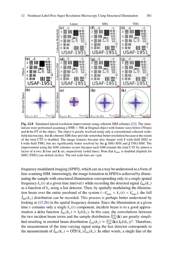
Fig. 12.8 Simulated lateral resolution improvement using coherent SIM schemes [23]. The simulations were performed assuming a SNR = 500. a Original object with feature sizes below (50 nm)
and b the FT of the object. The object is poorly resolved using only c conventional coherent widefield microscopy, but d coherent SIM does provide somewhat better resolution because e the extent
of the total CTF is doubled. The image features become also sharper with f wide-field SHG or
i wide-field THG, but are significantly better resolved by the g SHG-SIM and j THG-SIM. The
improvement using the SIM schemes occurs because each SIM extends the total CTF by almost a
factor of e two, h four and k six, respectively (solid lines). Note that k max is doubled (tripled) for
SHG (THG) (see dotted circles). The red scale bars are 1 µm
frequency modulated imaging (SPIFI), which can in a way be understood as a form of
line-scanning SIM. Interestingly, the image formation in SPIFI is achieved by illuminating the sample with structured illumination corresponding only to a single spatial
frequency k x (t) at a given time interval t while recording the detected signal ˆ
I det (k x )
as a function of k x using a fast detector. Then, by spatially modulating the illumination beam over the entire passband of the system (−k
max < k x (t) < k
max ), the full
ˆ
I det (k x ) distribution can be recorded. This process is perhaps better understood by
looking at (12.2b) in the spatial frequency domain. Since the illumination at a given
time t contains only a single k x (t) component, incident beam is to a good approximation a delta function ˆ
I inc (k x ) ≈ I 0 δ(k x ). In this case, the convolutions between
the two incident beam terms and the sample distribution ˆ
S
(2)
em (k) are greatly simplified resulting in emitted beam distribution ˆ
I em (k x ) ≈ ˆ
S
(2)
em (k)(I 0 δ(k x ))
2 . Therefore,
the measurement of the time-varying signal using the fast detector corresponds to
the measurement of ˆ
I det (k x ) = OTF(k x ) ˆ
I em (k x ). In other words, a single line of the
301
(a)
(c)
(d)
(e)
(f)
(g)
(h)
(i)
(j)
(k)
(b)
Fig. 12.8 Simulated lateral resolution improvement using coherent SIM schemes [23]. The simulations were performed assuming a SNR = 500. a Original object with feature sizes below (50 nm)
and b the FT of the object. The object is poorly resolved using only c conventional coherent widefield microscopy, but d coherent SIM does provide somewhat better resolution because e the extent
of the total CTF is doubled. The image features become also sharper with f wide-field SHG or
i wide-field THG, but are significantly better resolved by the g SHG-SIM and j THG-SIM. The
improvement using the SIM schemes occurs because each SIM extends the total CTF by almost a
factor of e two, h four and k six, respectively (solid lines). Note that k max is doubled (tripled) for
SHG (THG) (see dotted circles). The red scale bars are 1 µm
frequency modulated imaging (SPIFI), which can in a way be understood as a form of
line-scanning SIM. Interestingly, the image formation in SPIFI is achieved by illuminating the sample with structured illumination corresponding only to a single spatial
frequency k x (t) at a given time interval t while recording the detected signal ˆ
I det (k x )
as a function of k x using a fast detector. Then, by spatially modulating the illumination beam over the entire passband of the system (−k
max < k x (t) < k
max ), the full
ˆ
I det (k x ) distribution can be recorded. This process is perhaps better understood by
looking at (12.2b) in the spatial frequency domain. Since the illumination at a given
time t contains only a single k x (t) component, incident beam is to a good approximation a delta function ˆ
I inc (k x ) ≈ I 0 δ(k x ). In this case, the convolutions between
the two incident beam terms and the sample distribution ˆ
S
(2)
em (k) are greatly simplified resulting in emitted beam distribution ˆ
I em (k x ) ≈ ˆ
S
(2)
em (k)(I 0 δ(k x ))
2 . Therefore,
the measurement of the time-varying signal using the fast detector corresponds to
the measurement of ˆ
I det (k x ) = OTF(k x ) ˆ
I em (k x ). In other words, a single line of the