

8
C. Hu and G. Popescu
Fig. 1.3 Main configurations of QPI: a off-axis and b phase shifting methods (Reprinted from [92]
with permission)
1.3.1 Off-axis Methods
In off-axis schemes, the tilted reference field and the sample field go through a
different path and reach the image plane at the same time (t − t R = 0), and the
resulting irradiance of this interferogram is given by
I (x, y) = |U i (x, y)|
2
+ |U R |
2
+ 2|U i (x, y)||U R | cos[kx + ϕ(x, y)]
(1.16)
In (1.16), k = ||k − k R | is the magnitude of the wavevector difference between the
image and reference field, which is assumed to be along the x-axis, acting as the carrier frequency. The recorded image is essentially interference fringes, whose shapes
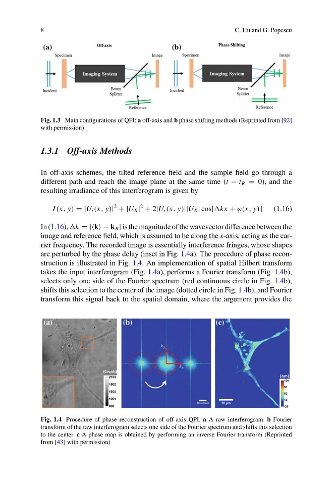
are perturbed by the phase delay (inset in Fig. 1.4a). The procedure of phase reconstruction is illustrated in Fig. 1.4. An implementation of spatial Hilbert transform
takes the input interferogram (Fig. 1.4a), performs a Fourier transform (Fig. 1.4b),
selects only one side of the Fourier spectrum (red continuous circle in Fig. 1.4b),
shifts this selection to the center of the image (dotted circle in Fig. 1.4b), and Fourier
transform this signal back to the spatial domain, where the argument provides the
Fig. 1.4 Procedure of phase reconstruction of off-axis QPI. a A raw interferogram. b Fourier
transform of the raw interferogram selects one side of the Fourier spectrum and shifts this selection
to the center. c A phase map is obtained by performing an inverse Fourier transform (Reprinted
from [43] with permission)
C. Hu and G. Popescu
Fig. 1.3 Main configurations of QPI: a off-axis and b phase shifting methods (Reprinted from [92]
with permission)
1.3.1 Off-axis Methods
In off-axis schemes, the tilted reference field and the sample field go through a
different path and reach the image plane at the same time (t − t R = 0), and the
resulting irradiance of this interferogram is given by
I (x, y) = |U i (x, y)|
2
+ |U R |
2
+ 2|U i (x, y)||U R | cos[kx + ϕ(x, y)]
(1.16)
In (1.16), k = ||k − k R | is the magnitude of the wavevector difference between the
image and reference field, which is assumed to be along the x-axis, acting as the carrier frequency. The recorded image is essentially interference fringes, whose shapes
are perturbed by the phase delay (inset in Fig. 1.4a). The procedure of phase reconstruction is illustrated in Fig. 1.4. An implementation of spatial Hilbert transform
takes the input interferogram (Fig. 1.4a), performs a Fourier transform (Fig. 1.4b),
selects only one side of the Fourier spectrum (red continuous circle in Fig. 1.4b),
shifts this selection to the center of the image (dotted circle in Fig. 1.4b), and Fourier
transform this signal back to the spatial domain, where the argument provides the
Fig. 1.4 Procedure of phase reconstruction of off-axis QPI. a A raw interferogram. b Fourier
transform of the raw interferogram selects one side of the Fourier spectrum and shifts this selection
to the center. c A phase map is obtained by performing an inverse Fourier transform (Reprinted
from [43] with permission)