

1 Quantitative Phase Imaging: Principles and Applications
7
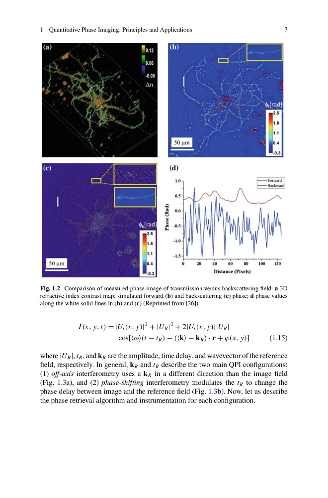
Fig. 1.2 Comparison of measured phase image of transmission versus backscattering field. a 3D
refractive index contrast map; simulated forward (b) and backscattering (c) phase; d phase values
along the white solid lines in (b) and (c) (Reprinted from [26])
I (x, y, t) = |U i (x, y)|
2
+ |U R |
2
+ 2|U i (x, y)||U R |
cos[ω(t − t R ) − (k − k R ) · r + ϕ(x, y)]
(1.15)
where |U R |, t R , and k R are the amplitude, time delay, and wavevector of the reference
field, respectively. In general, k R and t R describe the two main QPI configurations:
(1) off-axis interferometry uses a k R in a different direction than the image field
(Fig. 1.3a), and (2) phase-shifting interferometry modulates the t R to change the
phase delay between image and the reference field (Fig. 1.3b). Now, let us describe
the phase retrieval algorithm and instrumentation for each configuration.
7
Fig. 1.2 Comparison of measured phase image of transmission versus backscattering field. a 3D
refractive index contrast map; simulated forward (b) and backscattering (c) phase; d phase values
along the white solid lines in (b) and (c) (Reprinted from [26])
I (x, y, t) = |U i (x, y)|
2
+ |U R |
2
+ 2|U i (x, y)||U R |
cos[ω(t − t R ) − (k − k R ) · r + ϕ(x, y)]
(1.15)
where |U R |, t R , and k R are the amplitude, time delay, and wavevector of the reference
field, respectively. In general, k R and t R describe the two main QPI configurations:
(1) off-axis interferometry uses a k R in a different direction than the image field
(Fig. 1.3a), and (2) phase-shifting interferometry modulates the t R to change the
phase delay between image and the reference field (Fig. 1.3b). Now, let us describe
the phase retrieval algorithm and instrumentation for each configuration.