

6
C. Hu and G. Popescu
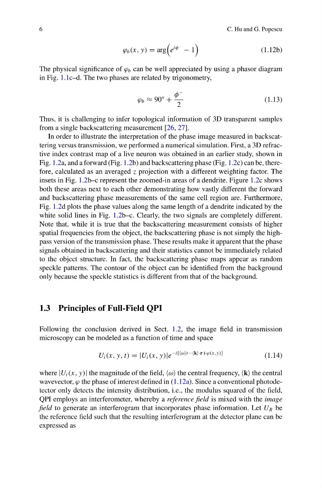
ϕ b (x, y) = arg
e
iφ
− − 1
(1.12b)
The physical significance of ϕ b can be well appreciated by using a phasor diagram
in Fig. 1.1c–d. The two phases are related by trigonometry,
ϕ b ≈ 90
◦
+
φ
−
2
(1.13)
Thus, it is challenging to infer topological information of 3D transparent samples
from a single backscattering measurement [26, 27].
In order to illustrate the interpretation of the phase image measured in backscattering versus transmission, we performed a numerical simulation. First, a 3D refractive index contrast map of a live neuron was obtained in an earlier study, shown in
Fig. 1.2a, and a forward (Fig. 1.2b) and backscattering phase (Fig. 1.2c) can be, therefore, calculated as an averaged z projection with a different weighting factor. The
insets in Fig. 1.2b–c represent the zoomed-in areas of a dendrite. Figure 1.2c shows
both these areas next to each other demonstrating how vastly different the forward
and backscattering phase measurements of the same cell region are. Furthermore,
Fig. 1.2d plots the phase values along the same length of a dendrite indicated by the
white solid lines in Fig. 1.2b–c. Clearly, the two signals are completely different.
Note that, while it is true that the backscattering measurement consists of higher
spatial frequencies from the object, the backscattering phase is not simply the highpass version of the transmission phase. These results make it apparent that the phase
signals obtained in backscattering and their statistics cannot be immediately related
to the object structure. In fact, the backscattering phase maps appear as random
speckle patterns. The contour of the object can be identified from the background
only because the speckle statistics is different from that of the background.
1.3 Principles of Full-Field QPI
Following the conclusion derived in Sect. 1.2, the image field in transmission
microscopy can be modeled as a function of time and space
U i (x, y, t) = |U i (x, y)|e
−i[ωt−k·r+ϕ(x,y)]
(1.14)
where |U i (x, y)| the magnitude of the field, ω the central frequency, k the central
wavevector, ϕ the phase of interest defined in (1.12a). Since a conventional photodetector only detects the intensity distribution, i.e., the modulus squared of the field,
QPI employs an interferometer, whereby a reference field is mixed with the image
field to generate an interferogram that incorporates phase information. Let U R be
the reference field such that the resulting interferogram at the detector plane can be
expressed as
C. Hu and G. Popescu
ϕ b (x, y) = arg
e
iφ
− − 1
(1.12b)
The physical significance of ϕ b can be well appreciated by using a phasor diagram
in Fig. 1.1c–d. The two phases are related by trigonometry,
ϕ b ≈ 90
◦
+
φ
−
2
(1.13)
Thus, it is challenging to infer topological information of 3D transparent samples
from a single backscattering measurement [26, 27].
In order to illustrate the interpretation of the phase image measured in backscattering versus transmission, we performed a numerical simulation. First, a 3D refractive index contrast map of a live neuron was obtained in an earlier study, shown in
Fig. 1.2a, and a forward (Fig. 1.2b) and backscattering phase (Fig. 1.2c) can be, therefore, calculated as an averaged z projection with a different weighting factor. The
insets in Fig. 1.2b–c represent the zoomed-in areas of a dendrite. Figure 1.2c shows
both these areas next to each other demonstrating how vastly different the forward
and backscattering phase measurements of the same cell region are. Furthermore,
Fig. 1.2d plots the phase values along the same length of a dendrite indicated by the
white solid lines in Fig. 1.2b–c. Clearly, the two signals are completely different.
Note that, while it is true that the backscattering measurement consists of higher
spatial frequencies from the object, the backscattering phase is not simply the highpass version of the transmission phase. These results make it apparent that the phase
signals obtained in backscattering and their statistics cannot be immediately related
to the object structure. In fact, the backscattering phase maps appear as random
speckle patterns. The contour of the object can be identified from the background
only because the speckle statistics is different from that of the background.
1.3 Principles of Full-Field QPI
Following the conclusion derived in Sect. 1.2, the image field in transmission
microscopy can be modeled as a function of time and space
U i (x, y, t) = |U i (x, y)|e
−i[ωt−k·r+ϕ(x,y)]
(1.14)
where |U i (x, y)| the magnitude of the field, ω the central frequency, k the central
wavevector, ϕ the phase of interest defined in (1.12a). Since a conventional photodetector only detects the intensity distribution, i.e., the modulus squared of the field,
QPI employs an interferometer, whereby a reference field is mixed with the image
field to generate an interferogram that incorporates phase information. Let U R be
the reference field such that the resulting interferogram at the detector plane can be
expressed as