

1 Quantitative Phase Imaging: Principles and Applications
5
U b (r ⊥ , z) = Ae
−iβz e
iβ 0
L / 2
−L / 2
[n(r ⊥ ,z)−n 0 ]e
i2βz dz
− Ae
−iβz
(1.11b)
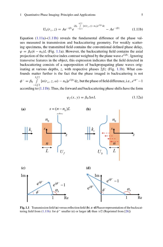
Equation (1.11a)–(1.11b) reveals the fundamental difference of the phase values measured in transmission and backscattering geometry. For weakly scattering specimens, the transmitted field contains the conventional defined phase delay,
ϕ = β 0 ( ¯
n − n 0 )L (Fig. 1.1a). However, the backscattering field contains the axial
projection of the refractive index contrast weighted by the plane wave e
i2βz . Ignoring
transverse features in the object, this expression indicates that the field detected in
backscattering consists of a superposition of backpropagating plane waves originating at various depths, z, with respective phases 2βz (Fig. 1.1b). What confounds matter further is the fact that the phase imaged in backscattering is not
φ
−
= β 0
L / 2
−L / 2
[n(r ⊥ , z, ω) − n 0 ]e
i2βz dz, but the phase of field difference, i.e., e
iφ
− −1
according to (1.11b). Thus, the forward and backscattering phase shifts have the form
ϕ f (x, y) = β 0 nL
(1.12a)
Fig. 1.1 Transmission field (a) versus reflection field (b). c–d Phasor representation of the backscattering field from (1.11b): for φ − smaller (c) or larger (d) than π/2 (Reprinted from [26])
5
U b (r ⊥ , z) = Ae
−iβz e
iβ 0
L / 2
−L / 2
[n(r ⊥ ,z)−n 0 ]e
i2βz dz
− Ae
−iβz
(1.11b)
Equation (1.11a)–(1.11b) reveals the fundamental difference of the phase values measured in transmission and backscattering geometry. For weakly scattering specimens, the transmitted field contains the conventional defined phase delay,
ϕ = β 0 ( ¯
n − n 0 )L (Fig. 1.1a). However, the backscattering field contains the axial
projection of the refractive index contrast weighted by the plane wave e
i2βz . Ignoring
transverse features in the object, this expression indicates that the field detected in
backscattering consists of a superposition of backpropagating plane waves originating at various depths, z, with respective phases 2βz (Fig. 1.1b). What confounds matter further is the fact that the phase imaged in backscattering is not
φ
−
= β 0
L / 2
−L / 2
[n(r ⊥ , z, ω) − n 0 ]e
i2βz dz, but the phase of field difference, i.e., e
iφ
− −1
according to (1.11b). Thus, the forward and backscattering phase shifts have the form
ϕ f (x, y) = β 0 nL
(1.12a)
Fig. 1.1 Transmission field (a) versus reflection field (b). c–d Phasor representation of the backscattering field from (1.11b): for φ − smaller (c) or larger (d) than π/2 (Reprinted from [26])