

4
C. Hu and G. Popescu
U
+
(r ⊥ , z) = −
i
2n 0
β 0 Ae
iβz
χ (r ⊥ , 0)
(1.7a)
U
−
(r ⊥ , z) =
i
2n 0
β 0 Ae
−iβz
χ (r ⊥ , −2β)
(1.7b)
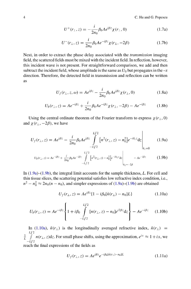
Next, in order to extract the phase delay associated with the transmission imaging
field, the scattered fields must be mixed with the incident field. In reflection, however,
this incident wave is not present. For straightforward comparison, we add and then
subtract the incident field, whose amplitude is the same as U 0 but propagates in the –z
direction. Therefore, the detected field in transmission and reflection can be written
as
U f (r ⊥ , z, ω) = Ae
iβz
−
i
2n 0
β 0 Ae
iβz
χ (r ⊥ , 0)
(1.8a)
U b (r ⊥ , z) = Ae
−iβz
+
i
2n 0
β 0 Ae
−iβz
χ (r ⊥ , −2β) − Ae
−iβz
(1.8b)
Using the central ordinate theorem of the Fourier transform to express χ(r ⊥ , 0)
and χ (r ⊥ , −2β), we have
U f (r ⊥ , z) = Ae
iβz
−
i
2n 0
β 0 Ae
iβz
L / 2
−L / 2
n
2
(r ⊥ , z) − n
2
0
e
−ik z z dz
k z =0
(1.9a)
U b (r ⊥ , z) = Ae −iβz +
i
2n 0
β 0 Ae −iβz
L
2
−L
2
n 2 (r ⊥ , z) − n 2
0
e −ikz z dz
kz =−2β
− Ae −iβz
(1.9b)
In (1.9a)–(1.9b), the integral limit accounts for the sample thickness, L. For cell and
thin tissue slices, the scattering potential satisfies low refractive index condition, i.e.,
n
2
− n
2
0 ≈ 2n 0 (n − n 0 ), and simpler expressions of (1.9a)–(1.9b) are obtained
U f (r ⊥ , z) = Ae
iβz
{1 − iβ 0 [ ¯
n(r ⊥ ) − n 0 ]L}
(1.10a)
U b (r ⊥ , z) = Ae
−iβz
⎧
⎪ ⎨
⎪ ⎩
1 + iβ 0
L / 2
−L / 2
[n(r ⊥ , z) − n 0 ]e
i2βz dz
⎫
⎪ ⎬
⎪ ⎭
− Ae
−iβz
(1.10b)
In (1.10a), ¯
n(r ⊥ ) is the longitudinally averaged refractive index, ¯
n(r ⊥ ) =
1
L
L / 2
−L / 2
n(r ⊥ , z)dz. For small phase shifts, using the approximation, e
i x
≈ 1 + i x, we
reach the final expressions of the fields as
U f (r ⊥ , z) = Ae
iβz e
−iβ 0 [ ¯
n(r ⊥ )−n0]L
(1.11a)
C. Hu and G. Popescu
U
+
(r ⊥ , z) = −
i
2n 0
β 0 Ae
iβz
χ (r ⊥ , 0)
(1.7a)
U
−
(r ⊥ , z) =
i
2n 0
β 0 Ae
−iβz
χ (r ⊥ , −2β)
(1.7b)
Next, in order to extract the phase delay associated with the transmission imaging
field, the scattered fields must be mixed with the incident field. In reflection, however,
this incident wave is not present. For straightforward comparison, we add and then
subtract the incident field, whose amplitude is the same as U 0 but propagates in the –z
direction. Therefore, the detected field in transmission and reflection can be written
as
U f (r ⊥ , z, ω) = Ae
iβz
−
i
2n 0
β 0 Ae
iβz
χ (r ⊥ , 0)
(1.8a)
U b (r ⊥ , z) = Ae
−iβz
+
i
2n 0
β 0 Ae
−iβz
χ (r ⊥ , −2β) − Ae
−iβz
(1.8b)
Using the central ordinate theorem of the Fourier transform to express χ(r ⊥ , 0)
and χ (r ⊥ , −2β), we have
U f (r ⊥ , z) = Ae
iβz
−
i
2n 0
β 0 Ae
iβz
L / 2
−L / 2
n
2
(r ⊥ , z) − n
2
0
e
−ik z z dz
k z =0
(1.9a)
U b (r ⊥ , z) = Ae −iβz +
i
2n 0
β 0 Ae −iβz
L
2
−L
2
n 2 (r ⊥ , z) − n 2
0
e −ikz z dz
kz =−2β
− Ae −iβz
(1.9b)
In (1.9a)–(1.9b), the integral limit accounts for the sample thickness, L. For cell and
thin tissue slices, the scattering potential satisfies low refractive index condition, i.e.,
n
2
− n
2
0 ≈ 2n 0 (n − n 0 ), and simpler expressions of (1.9a)–(1.9b) are obtained
U f (r ⊥ , z) = Ae
iβz
{1 − iβ 0 [ ¯
n(r ⊥ ) − n 0 ]L}
(1.10a)
U b (r ⊥ , z) = Ae
−iβz
⎧
⎪ ⎨
⎪ ⎩
1 + iβ 0
L / 2
−L / 2
[n(r ⊥ , z) − n 0 ]e
i2βz dz
⎫
⎪ ⎬
⎪ ⎭
− Ae
−iβz
(1.10b)
In (1.10a), ¯
n(r ⊥ ) is the longitudinally averaged refractive index, ¯
n(r ⊥ ) =
1
L
L / 2
−L / 2
n(r ⊥ , z)dz. For small phase shifts, using the approximation, e
i x
≈ 1 + i x, we
reach the final expressions of the fields as
U f (r ⊥ , z) = Ae
iβz e
−iβ 0 [ ¯
n(r ⊥ )−n0]L
(1.11a)