

1 Quantitative Phase Imaging: Principles and Applications
3
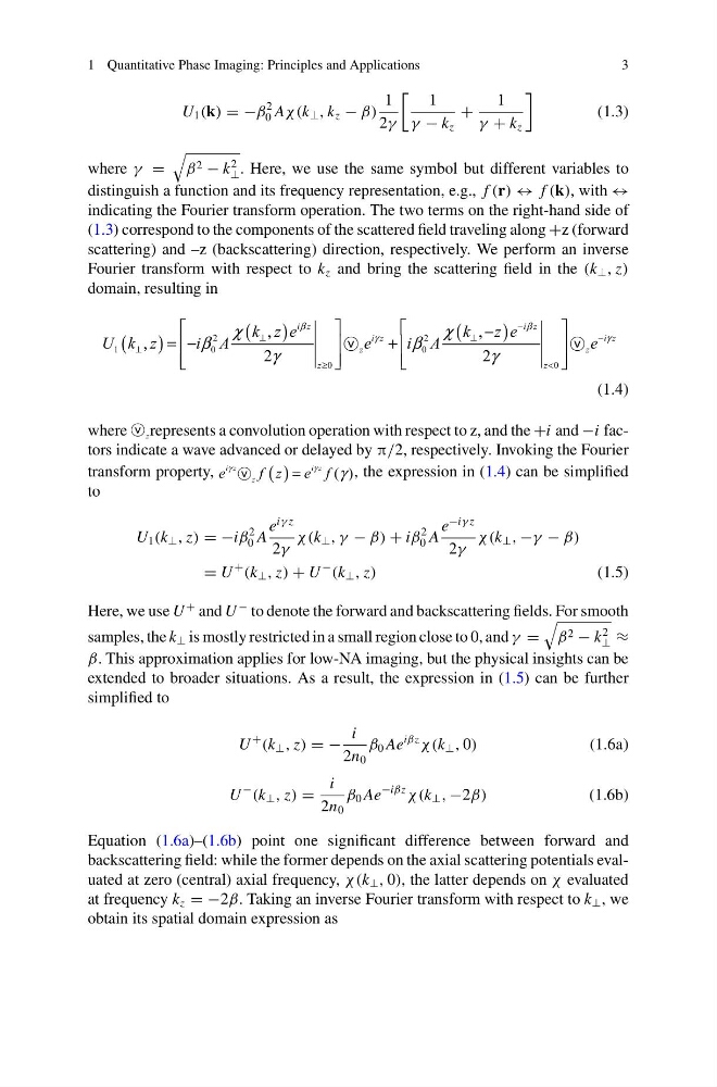
U 1 (k) = −β
2
0 Aχ (k ⊥ , k z − β)
1
2γ
1
γ − k z
+
1
γ + k z
(1.3)
where γ =
β 2 − k
2
⊥ . Here, we use the same symbol but different variables to
distinguish a function and its frequency representation, e.g., f (r) ↔ f (k), with ↔
indicating the Fourier transform operation. The two terms on the right-hand side of
(1.3) correspond to the components of the scattered field traveling along +z (forward
scattering) and –z (backscattering) direction, respectively. We perform an inverse
Fourier transform with respect to k z and bring the scattering field in the (k ⊥ , z)
domain, resulting in
( )
( )
(
)
2
2
1
0
0
0
0
,
,
,
2
2
i z
i z
i z
i z
z
z
z
z
k z e
k
z e
U k z
i A
e
i A
e
β
β
γ
γ
χ
χ
β
β
γ
γ
−
⊥
⊥
−
⊥
<
≥
⎡
⎤
⎡
⎤
−
= −
+
⎢
⎥
⎢
⎥
⎢
⎥
⎢
⎥
⎣
⎦
⎣
⎦
ⓥ
ⓥ
(1.4)
where z
ⓥ represents a convolution operation with respect to z, and the +i and −i factors indicate a wave advanced or delayed by π/2, respectively. Invoking the Fourier
transform property,
( )
( )
i z
i
z
z
f z
e
e f
γ
γ
=
ⓥ
γ , the expression in (1.4) can be simplified
to
U 1 (k ⊥ , z) = −iβ
2
0 A
e
iγ z
2γ
χ (k ⊥ , γ − β) + iβ
2
0 A
e
−iγ z
2γ
χ (k ⊥ , −γ − β)
= U
+
(k ⊥ , z) + U
−
(k ⊥ , z)
(1.5)
Here, we use U
+ and U
− to denote the forward and backscattering fields. For smooth
samples, the k ⊥ is mostly restricted in a small region close to 0, and γ =
β 2 − k
2
⊥ ≈
β. This approximation applies for low-NA imaging, but the physical insights can be
extended to broader situations. As a result, the expression in (1.5) can be further
simplified to
U
+
(k ⊥ , z) = −
i
2n 0
β 0 Ae
iβz
χ (k ⊥ , 0)
(1.6a)
U
−
(k ⊥ , z) =
i
2n 0
β 0 Ae
−iβz
χ (k ⊥ , −2β)
(1.6b)
Equation (1.6a)–(1.6b) point one significant difference between forward and
backscattering field: while the former depends on the axial scattering potentials evaluated at zero (central) axial frequency, χ (k ⊥ , 0), the latter depends on χ evaluated
at frequency k z = −2β. Taking an inverse Fourier transform with respect to k ⊥ , we
obtain its spatial domain expression as
3
U 1 (k) = −β
2
0 Aχ (k ⊥ , k z − β)
1
2γ
1
γ − k z
+
1
γ + k z
(1.3)
where γ =
β 2 − k
2
⊥ . Here, we use the same symbol but different variables to
distinguish a function and its frequency representation, e.g., f (r) ↔ f (k), with ↔
indicating the Fourier transform operation. The two terms on the right-hand side of
(1.3) correspond to the components of the scattered field traveling along +z (forward
scattering) and –z (backscattering) direction, respectively. We perform an inverse
Fourier transform with respect to k z and bring the scattering field in the (k ⊥ , z)
domain, resulting in
( )
( )
(
)
2
2
1
0
0
0
0
,
,
,
2
2
i z
i z
i z
i z
z
z
z
z
k z e
k
z e
U k z
i A
e
i A
e
β
β
γ
γ
χ
χ
β
β
γ
γ
−
⊥
⊥
−
⊥
<
≥
⎡
⎤
⎡
⎤
−
= −
+
⎢
⎥
⎢
⎥
⎢
⎥
⎢
⎥
⎣
⎦
⎣
⎦
ⓥ
ⓥ
(1.4)
where z
ⓥ represents a convolution operation with respect to z, and the +i and −i factors indicate a wave advanced or delayed by π/2, respectively. Invoking the Fourier
transform property,
( )
( )
i z
i
z
z
f z
e
e f
γ
γ
=
ⓥ
γ , the expression in (1.4) can be simplified
to
U 1 (k ⊥ , z) = −iβ
2
0 A
e
iγ z
2γ
χ (k ⊥ , γ − β) + iβ
2
0 A
e
−iγ z
2γ
χ (k ⊥ , −γ − β)
= U
+
(k ⊥ , z) + U
−
(k ⊥ , z)
(1.5)
Here, we use U
+ and U
− to denote the forward and backscattering fields. For smooth
samples, the k ⊥ is mostly restricted in a small region close to 0, and γ =
β 2 − k
2
⊥ ≈
β. This approximation applies for low-NA imaging, but the physical insights can be
extended to broader situations. As a result, the expression in (1.5) can be further
simplified to
U
+
(k ⊥ , z) = −
i
2n 0
β 0 Ae
iβz
χ (k ⊥ , 0)
(1.6a)
U
−
(k ⊥ , z) =
i
2n 0
β 0 Ae
−iβz
χ (k ⊥ , −2β)
(1.6b)
Equation (1.6a)–(1.6b) point one significant difference between forward and
backscattering field: while the former depends on the axial scattering potentials evaluated at zero (central) axial frequency, χ (k ⊥ , 0), the latter depends on χ evaluated
at frequency k z = −2β. Taking an inverse Fourier transform with respect to k ⊥ , we
obtain its spatial domain expression as