

280
A. Wittek et al.
I =
D
f (x) dD,
(11.16)
I ∼ = Q n (D) =
n
i=1
w i f (x i ) ,
(11.17)
where f is the function we intend to integrate, I is the integral approximated using
the n-point Gaussian quadrature Q n over the integration cell D, x i is the integration
points and w i is the corresponding weights
2. Nodal integration where the interpolating nodes are also used as integration
points [36, 37]
As the literature indicates that Gaussian quadrature over the background integration cells tends to be less computationally demanding than nodal integration
schemes [38], in the Meshless Total Lagrangian Explicit Dynamics (MTLED)
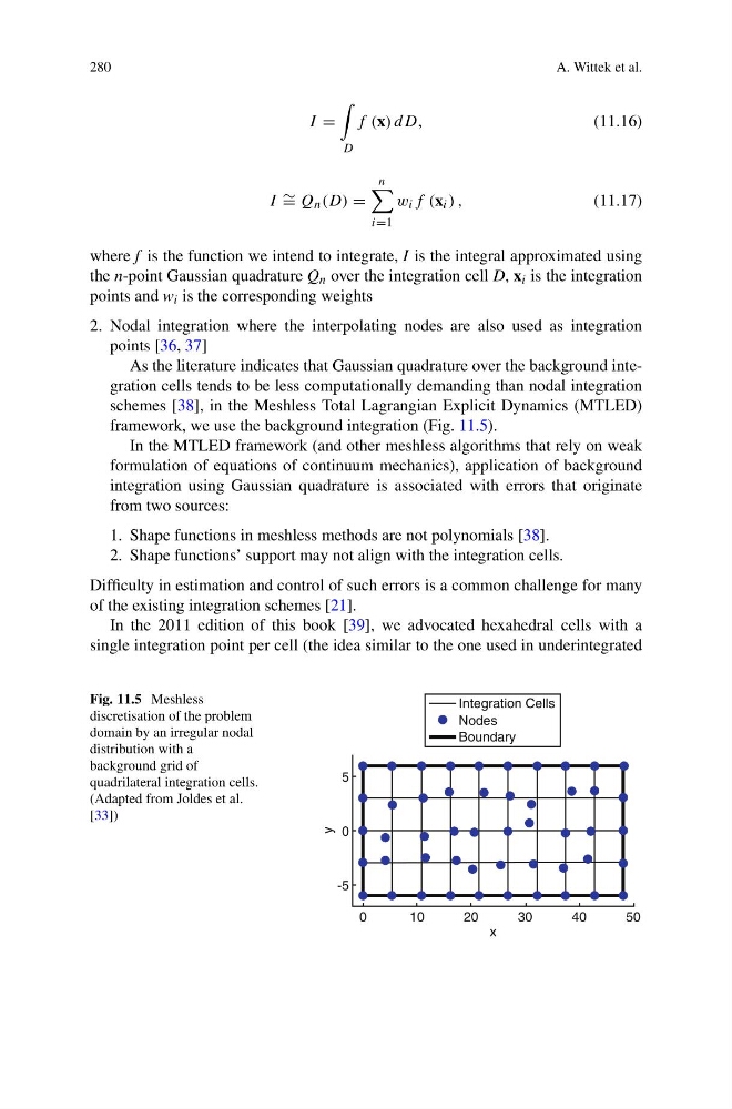
framework, we use the background integration (Fig. 11.5).
In the MTLED framework (and other meshless algorithms that rely on weak
formulation of equations of continuum mechanics), application of background
integration using Gaussian quadrature is associated with errors that originate
from two sources:
1. Shape functions in meshless methods are not polynomials [38].
2. Shape functions’ support may not align with the integration cells.
Difficulty in estimation and control of such errors is a common challenge for many
of the existing integration schemes [21].
In the 2011 edition of this book [39], we advocated hexahedral cells with a
single integration point per cell (the idea similar to the one used in underintegrated
Fig. 11.5 Meshless
discretisation of the problem
domain by an irregular nodal
distribution with a
background grid of
quadrilateral integration cells.
(Adapted from Joldes et al.
[33])
Integration Cells
Nodes
Boundary
5
-5
0
0
1 0
2 0
x
y
30
40
50
A. Wittek et al.
I =
D
f (x) dD,
(11.16)
I ∼ = Q n (D) =
n
i=1
w i f (x i ) ,
(11.17)
where f is the function we intend to integrate, I is the integral approximated using
the n-point Gaussian quadrature Q n over the integration cell D, x i is the integration
points and w i is the corresponding weights
2. Nodal integration where the interpolating nodes are also used as integration
points [36, 37]
As the literature indicates that Gaussian quadrature over the background integration cells tends to be less computationally demanding than nodal integration
schemes [38], in the Meshless Total Lagrangian Explicit Dynamics (MTLED)
framework, we use the background integration (Fig. 11.5).
In the MTLED framework (and other meshless algorithms that rely on weak
formulation of equations of continuum mechanics), application of background
integration using Gaussian quadrature is associated with errors that originate
from two sources:
1. Shape functions in meshless methods are not polynomials [38].
2. Shape functions’ support may not align with the integration cells.
Difficulty in estimation and control of such errors is a common challenge for many
of the existing integration schemes [21].
In the 2011 edition of this book [39], we advocated hexahedral cells with a
single integration point per cell (the idea similar to the one used in underintegrated
Fig. 11.5 Meshless
discretisation of the problem
domain by an irregular nodal
distribution with a
background grid of
quadrilateral integration cells.
(Adapted from Joldes et al.
[33])
Integration Cells
Nodes
Boundary
5
-5
0
0
1 0
2 0
x
y
30
40
50