

276
A. Wittek et al.
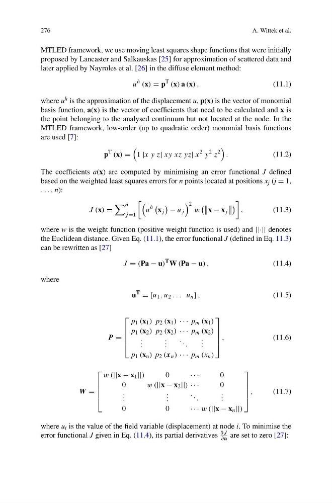
MTLED framework, we use moving least squares shape functions that were initially
proposed by Lancaster and Salkauskas [25] for approximation of scattered data and
later applied by Nayroles et al. [26] in the diffuse element method:
u
h (x) = p
T (x) a (x) ,
(11.1)
where u h is the approximation of the displacement u, p(x) is the vector of monomial
basis function, a(x) is the vector of coefficients that need to be calculated and x is
the point belonging to the analysed continuum but not located at the node. In the
MTLED framework, low-order (up to quadratic order) monomial basis functions
are used [7]:
p
T (x) =
1 |x y z| xy xz yz| x
2 y
2 z
2
.
(11.2)
The coefficients a(x) are computed by minimising an error functional J defined
based on the weighted least squares errors for n points located at positions x j (j = 1,
. . . , n):
J (x) =
n
j =1
u
h
x j
− u j
2
w
x − x j
,
(11.3)
where w is the weight function (positive weight function is used) and ||·|| denotes
the Euclidean distance. Given Eq. (11.1), the error functional J (defined in Eq. 11.3)
can be rewritten as [27]
J = (Pa − u)
T W (Pa − u) ,
(11.4)
where
u
T
= [u 1 , u 2 . . . u n ] ,
(11.5)
P =
⎡
⎢
⎢
⎢
⎣
p 1 (x 1 ) p 2 (x 1 ) · · · p m (x 1 )
p 1 (x 2 ) p 2 (x 2 ) · · · p m (x 2 )
. . .
. . .
. . .
. . .
p 1 (x n ) p 2 (x n ) · · · p m (x n )
⎤
⎥
⎥
⎥
⎦
,
(11.6)
W =
⎡
⎢
⎢
⎢
⎣
w (||x − x 1 ||)
0
· · ·
0
0
w (||x − x 2 ||) · · ·
0
. . .
. . .
. . .
. . .
0
0
· · · w (||x − x n ||)
⎤
⎥
⎥
⎥
⎦
,
(11.7)
where u i is the value of the field variable (displacement) at node i. To minimise the
error functional J given in Eq. (11.4), its partial derivatives
∂J
∂a are set to zero [27]:
A. Wittek et al.
MTLED framework, we use moving least squares shape functions that were initially
proposed by Lancaster and Salkauskas [25] for approximation of scattered data and
later applied by Nayroles et al. [26] in the diffuse element method:
u
h (x) = p
T (x) a (x) ,
(11.1)
where u h is the approximation of the displacement u, p(x) is the vector of monomial
basis function, a(x) is the vector of coefficients that need to be calculated and x is
the point belonging to the analysed continuum but not located at the node. In the
MTLED framework, low-order (up to quadratic order) monomial basis functions
are used [7]:
p
T (x) =
1 |x y z| xy xz yz| x
2 y
2 z
2
.
(11.2)
The coefficients a(x) are computed by minimising an error functional J defined
based on the weighted least squares errors for n points located at positions x j (j = 1,
. . . , n):
J (x) =
n
j =1
u
h
x j
− u j
2
w
x − x j
,
(11.3)
where w is the weight function (positive weight function is used) and ||·|| denotes
the Euclidean distance. Given Eq. (11.1), the error functional J (defined in Eq. 11.3)
can be rewritten as [27]
J = (Pa − u)
T W (Pa − u) ,
(11.4)
where
u
T
= [u 1 , u 2 . . . u n ] ,
(11.5)
P =
⎡
⎢
⎢
⎢
⎣
p 1 (x 1 ) p 2 (x 1 ) · · · p m (x 1 )
p 1 (x 2 ) p 2 (x 2 ) · · · p m (x 2 )
. . .
. . .
. . .
. . .
p 1 (x n ) p 2 (x n ) · · · p m (x n )
⎤
⎥
⎥
⎥
⎦
,
(11.6)
W =
⎡
⎢
⎢
⎢
⎣
w (||x − x 1 ||)
0
· · ·
0
0
w (||x − x 2 ||) · · ·
0
. . .
. . .
. . .
. . .
0
0
· · · w (||x − x n ||)
⎤
⎥
⎥
⎥
⎦
,
(11.7)
where u i is the value of the field variable (displacement) at node i. To minimise the
error functional J given in Eq. (11.4), its partial derivatives
∂J
∂a are set to zero [27]: