

3.6 Scattering Matrix
53
1
1.1
1.2
1.3
1.4
1.5
1.6
1.7
1.8
1.9
2
10
-14
10
-12
10
-10
10
-8
10
-6
10
-4
10
-2
10
0
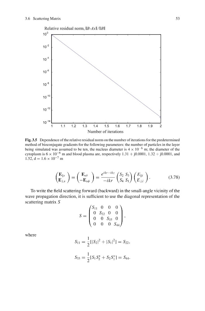
Fig. 3.5 Dependence of the relative residual norm on the number of iterations for the predetermined
method of bioconjugate gradients for the following parameters: the number of particles in the layer
being simulated was assumed to be ten, the nucleus diameter is 4 × 10 −6 m; the diameter of the
cytoplasm is 6 × 10 −6 m and blood plasma are, respectively 1.31 + j0.0001, 1.32 + j0.0001, and
1.52, d = 1.6 × 10 −7 m
E s
E ⊥s
=
E sθ
−E sφ
=
e
ikr−ikz
−ikr
S 2 S 3
S 4 S 1
E i
E ⊥i
.
(3.78)
To write the field scattering forward (backward) in the small-angle vicinity of the
wave propagation direction, it is sufficient to use the diagonal representation of the
scattering matrix S
S =
⎛
⎜
⎜
⎝
S 11 0 0 0
0 S 22 0 0
0 0 S 33 0
0 0 0 S 44
⎞
⎟
⎟
⎠ ,
where
S 11 =
1
2
[|S 2 |
2
+ |S 1 |
2
] = S 22 ,
S 33 =
1
2
[S 1 S
∗
2 + S 2 S
∗
1 ] = S 44 .
53
1
1.1
1.2
1.3
1.4
1.5
1.6
1.7
1.8
1.9
2
10
-14
10
-12
10
-10
10
-8
10
-6
10
-4
10
-2
10
0
Fig. 3.5 Dependence of the relative residual norm on the number of iterations for the predetermined
method of bioconjugate gradients for the following parameters: the number of particles in the layer
being simulated was assumed to be ten, the nucleus diameter is 4 × 10 −6 m; the diameter of the
cytoplasm is 6 × 10 −6 m and blood plasma are, respectively 1.31 + j0.0001, 1.32 + j0.0001, and
1.52, d = 1.6 × 10 −7 m
E s
E ⊥s
=
E sθ
−E sφ
=
e
ikr−ikz
−ikr
S 2 S 3
S 4 S 1
E i
E ⊥i
.
(3.78)
To write the field scattering forward (backward) in the small-angle vicinity of the
wave propagation direction, it is sufficient to use the diagonal representation of the
scattering matrix S
S =
⎛
⎜
⎜
⎝
S 11 0 0 0
0 S 22 0 0
0 0 S 33 0
0 0 0 S 44
⎞
⎟
⎟
⎠ ,
where
S 11 =
1
2
[|S 2 |
2
+ |S 1 |
2
] = S 22 ,
S 33 =
1
2
[S 1 S
∗
2 + S 2 S
∗
1 ] = S 44 .