

2.3 Stationary Theory of Radiative Transfer
13
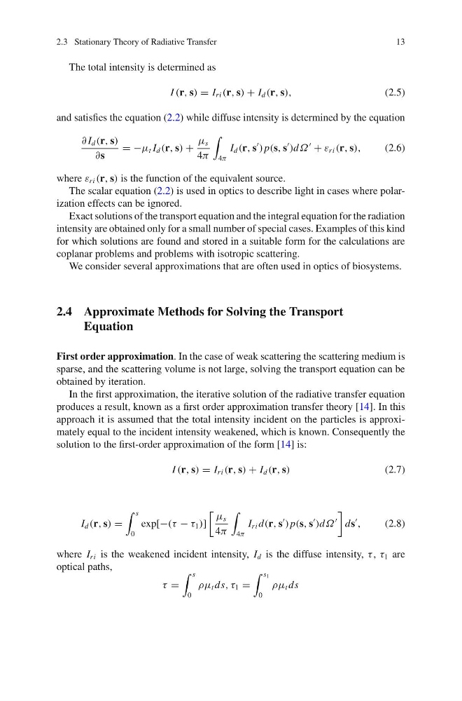
The total intensity is determined as
I (r, s) = I ri (r, s) + I d (r, s),
(2.5)
and satisfies the equation (2.2) while diffuse intensity is determined by the equation
∂ I d (r, s)
∂s
= −μ t I d (r, s) +
μ s
4π
4π
I d (r, s
) p(s, s
)dΩ
+ ε ri (r, s),
(2.6)
where ε ri (r, s) is the function of the equivalent source.
The scalar equation (2.2) is used in optics to describe light in cases where polarization effects can be ignored.
Exact solutions of the transport equation and the integral equation for the radiation
intensity are obtained only for a small number of special cases. Examples of this kind
for which solutions are found and stored in a suitable form for the calculations are
coplanar problems and problems with isotropic scattering.
We consider several approximations that are often used in optics of biosystems.
2.4 Approximate Methods for Solving the Transport
Equation
First order approximation. In the case of weak scattering the scattering medium is
sparse, and the scattering volume is not large, solving the transport equation can be
obtained by iteration.
In the first approximation, the iterative solution of the radiative transfer equation
produces a result, known as a first order approximation transfer theory [14]. In this
approach it is assumed that the total intensity incident on the particles is approximately equal to the incident intensity weakened, which is known. Consequently the
solution to the first-order approximation of the form [14] is:
I (r, s) = I ri (r, s) + I d (r, s)
(2.7)
I d (r, s) =
s
0
exp[−(τ − τ 1 )]
μ s
4π
4π
I ri d(r, s
) p(s, s
)dΩ
ds
,
(2.8)
where I ri is the weakened incident intensity, I d is the diffuse intensity, τ , τ 1 are
optical paths,
τ =
s
0
ρμ t ds, τ 1 =
s 1
0
ρμ t ds
13
The total intensity is determined as
I (r, s) = I ri (r, s) + I d (r, s),
(2.5)
and satisfies the equation (2.2) while diffuse intensity is determined by the equation
∂ I d (r, s)
∂s
= −μ t I d (r, s) +
μ s
4π
4π
I d (r, s
) p(s, s
)dΩ
+ ε ri (r, s),
(2.6)
where ε ri (r, s) is the function of the equivalent source.
The scalar equation (2.2) is used in optics to describe light in cases where polarization effects can be ignored.
Exact solutions of the transport equation and the integral equation for the radiation
intensity are obtained only for a small number of special cases. Examples of this kind
for which solutions are found and stored in a suitable form for the calculations are
coplanar problems and problems with isotropic scattering.
We consider several approximations that are often used in optics of biosystems.
2.4 Approximate Methods for Solving the Transport
Equation
First order approximation. In the case of weak scattering the scattering medium is
sparse, and the scattering volume is not large, solving the transport equation can be
obtained by iteration.
In the first approximation, the iterative solution of the radiative transfer equation
produces a result, known as a first order approximation transfer theory [14]. In this
approach it is assumed that the total intensity incident on the particles is approximately equal to the incident intensity weakened, which is known. Consequently the
solution to the first-order approximation of the form [14] is:
I (r, s) = I ri (r, s) + I d (r, s)
(2.7)
I d (r, s) =
s
0
exp[−(τ − τ 1 )]
μ s
4π
4π
I ri d(r, s
) p(s, s
)dΩ
ds
,
(2.8)
where I ri is the weakened incident intensity, I d is the diffuse intensity, τ , τ 1 are
optical paths,
τ =
s
0
ρμ t ds, τ 1 =
s 1
0
ρμ t ds